Bayes news: teaching the Beta-Binomial using real and fake headlines
UKCOTS 2025 University of Glasgow
Dr. Laurie Baker, Bates College; Dr. Jim Scott, Colby College; Dr. Mine Dogucu, UC Irvine
Outline
Introduce the Course Context
Introduce the Activity
Next Steps
Course Context
Target Course: Intro to Probability and Statistics or Bayesian Statistics Course
Student Background:
Basic probability concepts (e.g., probability of success/failure)
What a probability distribution represents
Familiarity with the concept of conditional probability
Some prior experience with R programming
Activity Overview
Goal: Show how priors, data, and posteriors interact with a real example
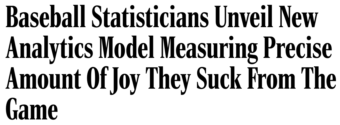
CNN (the Cable News Network) is widely considered a reputable news source. The Onion, on the other hand, is (according to Wikipedia) “an American news satire organization.
How well do people distinguish real news stories published on cnn.com from fake news stories published on theonion.com?
Learning Objectives
Define and distinguish between prior and posterior distributions.
Use the Beta distribution to construct prior beliefs about a probability.
Apply Bayesian updating to revise beliefs with observed data.
Interpret summary statistics (mean, mode, standard deviation) of Beta distributions.
Reflect on how prior information and data interact to shape posterior conclusions.
Activity Sequence
Introduce the Context
Construct and Visualize Priors
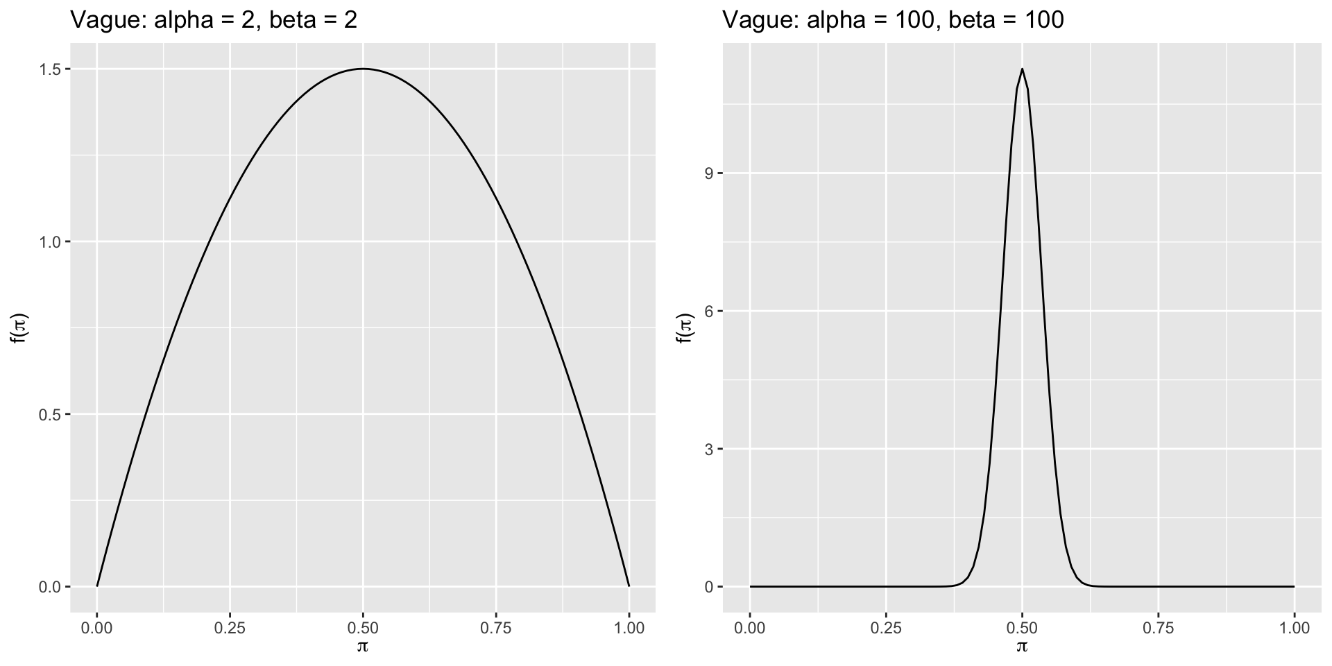
Discuss Vague vs. Informative Priors
Take the Quiz
Update Priors with Data and Visualize Posterior
Update Priors with Class Data and Visualize Posterior
Compare Posteriors from Different Priors
Discussion questions
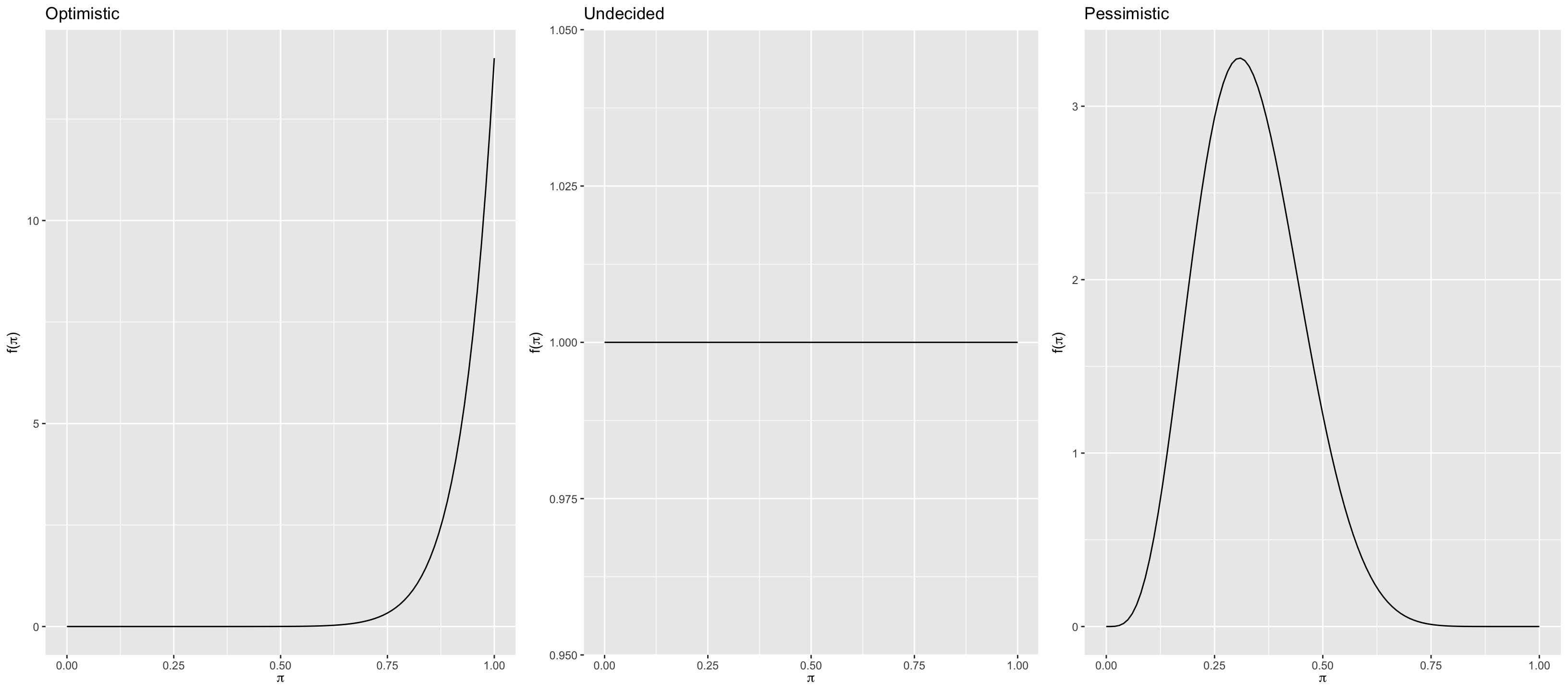
1. Introduce priors
Let \(\pi\) be the proportion of correct answers a person guesses right in the CNN vs the Onion quiz.
Optimistic
Undecided
Pessimistic
Beta(14, 1)
Beta(1, 1)
Beta(5, 10)
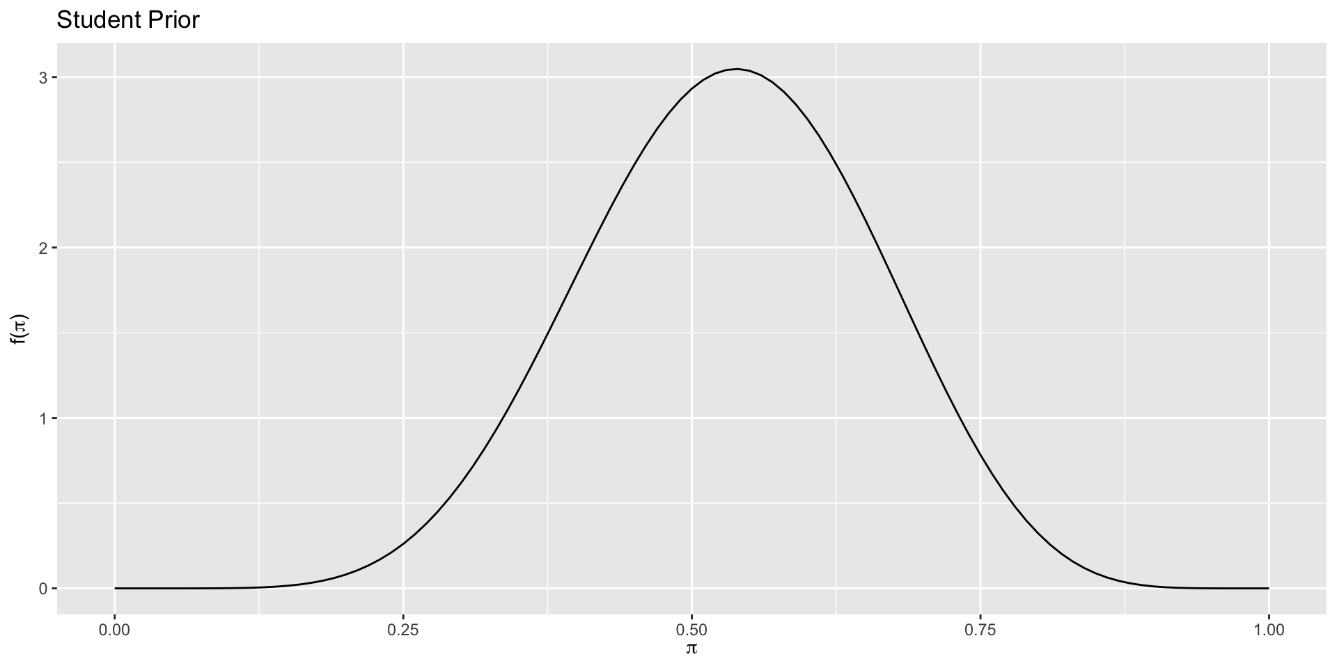
2. Constructing priors
The shape parameters \(\alpha\) and \(\beta\) can be interpreted as the approximate number of successes and failures.
summarize_beta_binomial(alpha, beta, y = NULL, n = NULL) summarizes the mean, mode, and variance of the prior and posterior Beta models of \(\pi\)
plot_beta_binomial(alpha, beta, y = NULL, n = NULL) [function produces a plot of any combination of the corresponding]; plots prior pdf, scaled likelihood function, and posterior pdf
Arguments:
-   `alpha, beta`: positive shape parameters of the prior Beta model
-   `y`: number of successes
-   `n`: number of trials
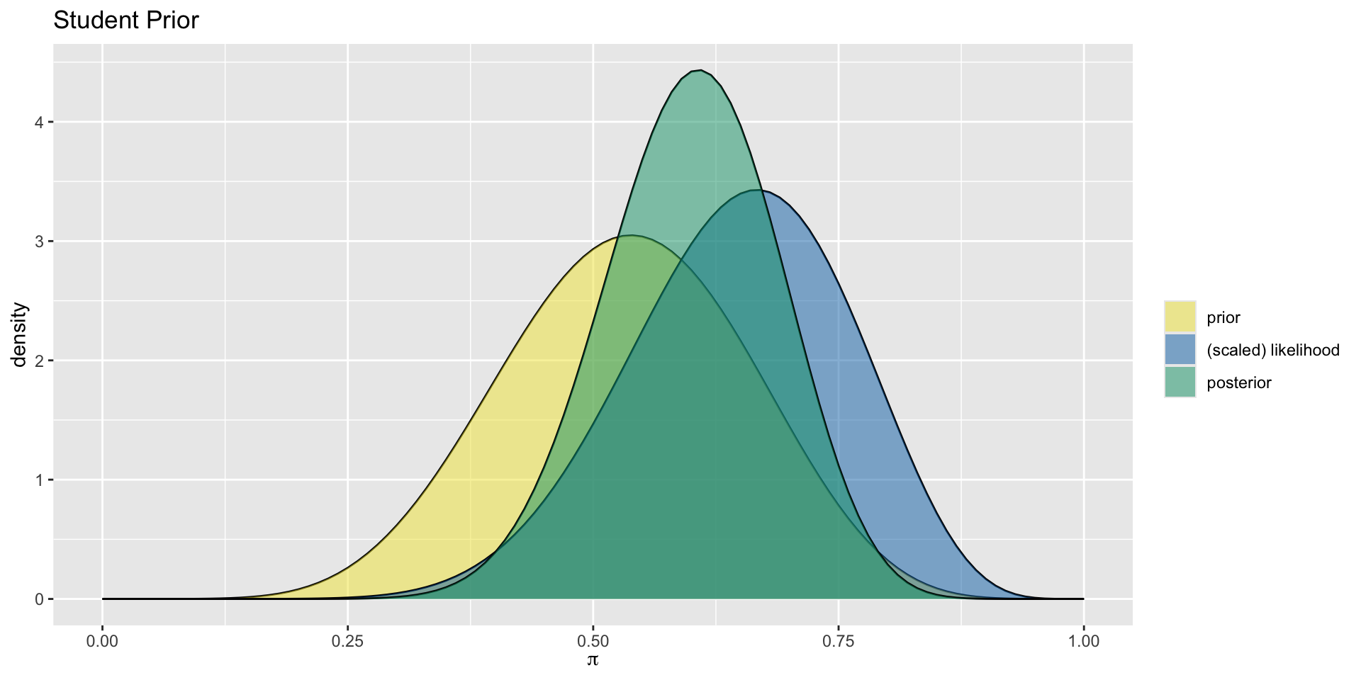
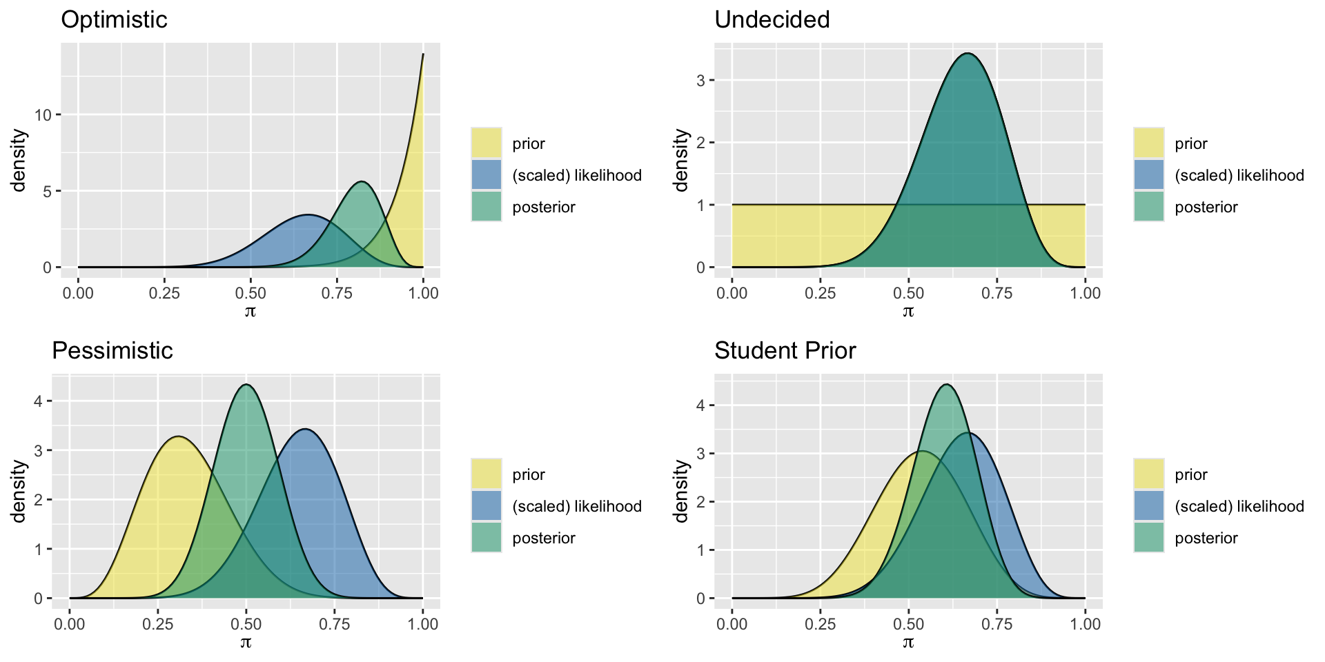
5. Update with data
summarize_beta_binomial(alpha =8, beta =7, y =10, n =15)
      model alpha beta      mean      mode         var         sd
1     prior     8    7 0.5333333 0.5384615 0.015555556 0.12472191
2 posterior    18   12 0.6000000 0.6071429 0.007741935 0.08798827
plot_beta_binomial(alpha =8, beta =7, y =10, n =15) +labs(title ="Student Prior")
5. Update with data
Optimistic
Undecided
Pessimistic
Student Prior
Beta(14, 1)
Beta(1, 1)
Beta(5, 10)
Beta(8, 7)
optimistic_prior <-plot_beta_binomial(alpha =14, beta =1, y =10, n =15) +labs(title ="Optimistic")undecided_prior <-plot_beta_binomial(alpha =1, beta =1, y =10, n =15) +labs(title ="Undecided")pessimistic_prior <-plot_beta_binomial(alpha =5, beta =10, y =10, n =15) +labs(title ="Pessimistic")student_prior <-plot_beta_binomial(alpha =8, beta =7, y =10, n =15) +labs(title ="Student Prior")
5. Update with data
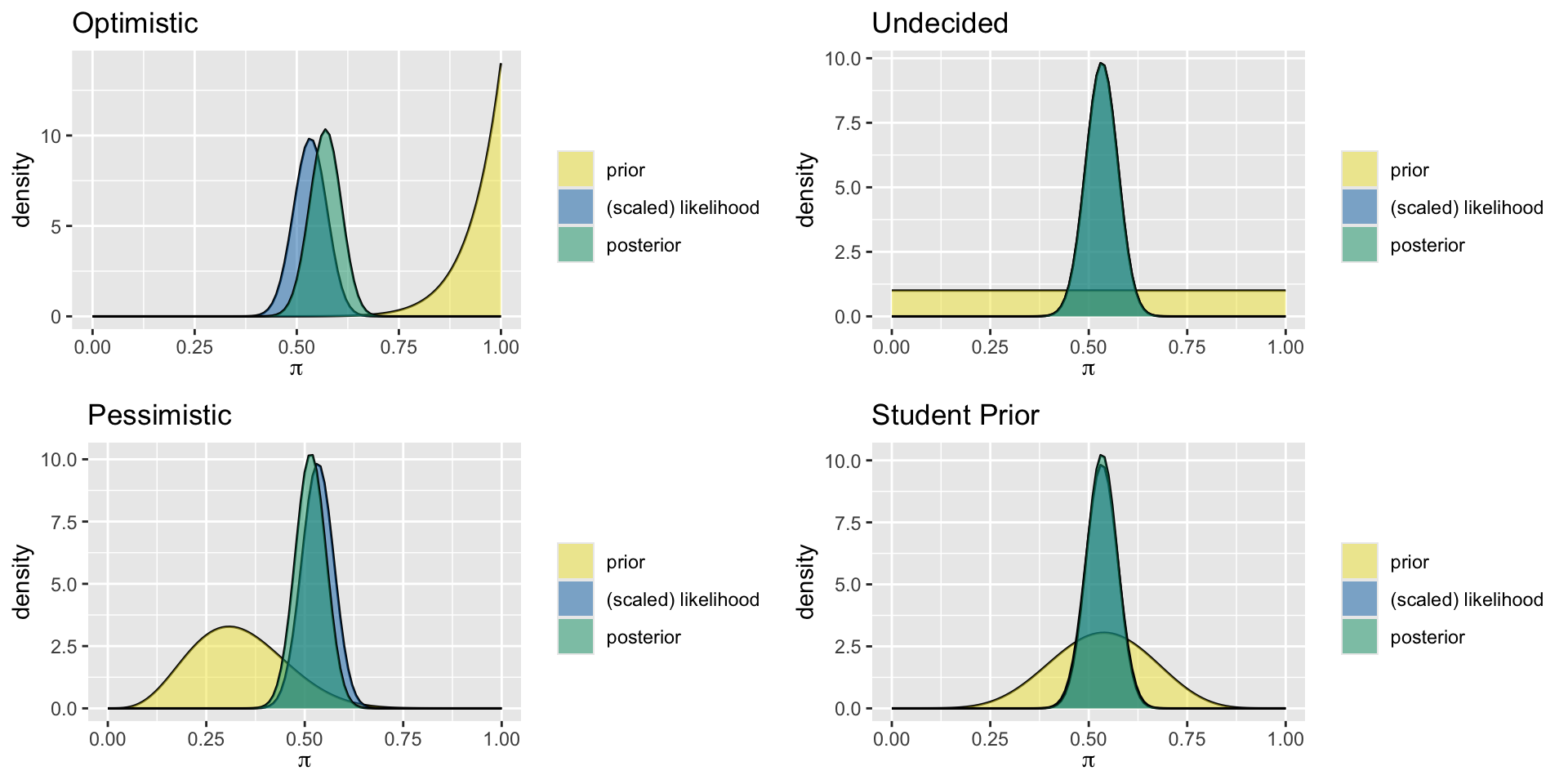
6. Update with neighbor and class data
With class data: 80 correct out of 150 questions
Optimistic
Undecided
Pessimistic
Student Prior
Beta(14, 1)
Beta(1, 1)
Beta(5, 10)
Beta(8, 7)
optimist <-plot_beta_binomial(alpha =14, beta =1, y =80, n =150) +labs(title ="Optimistic")undecided <-plot_beta_binomial(alpha =1, beta =1, y =80, n =150) +labs(title ="Undecided")pessimist <-plot_beta_binomial(alpha =5, beta =10, y =80, n =150) +labs(title ="Pessimistic")student_prior <-plot_beta_binomial(alpha =8, beta =7, y =80, n =150) +labs(title ="Student Prior")
7. Compare effects of prior choice on the posterior
8. Discussion Questions
How does observing more data affect the shape of the posterior?
What happens to the posterior mean as you observe more correct or incorrect outcomes?
In what ways does the posterior reflect a compromise between prior belief and observed data?

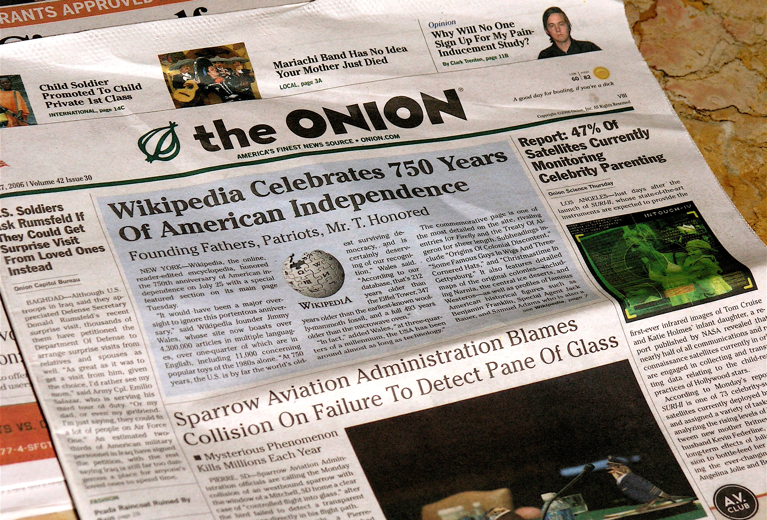 CNN (the Cable News Network) is widely considered a reputable news source. The Onion, on the other hand, is (according to Wikipedia) “an American news satire organization.