Inference: frequentist vs. Bayesian

Day 5

“Statistical inference”

• Hypothesis Testing a la frequentist

• Confidence Intervals

• Hypothesis Testing a la Bayes

• Credible Intervals

Resources

• Frequentist examples are from stats4cs.com

• Bayesian examples are from Bayes Rules! Section 8.2

Frequentist Inference

Research Question

Are there any pink cows in the world?

Hypotheses

Null hypothesis: There are no pink cows in the world.

Alternative hypothesis: There is a pink cow in the world.

Hypothesis Testing Procedure

We go looking for evidence against the null.

• If we find any evidence against the null (a single pink cow) then we say we reject the null hypothesis.

• If we do not find any evidence against the null (a single pink cow) then we fail to reject the null. We can keep searching for more evidence against the null (i.e. continue looking for a pink cow). We will never be able to say the null is true so we never accept the null. All we can do is keep looking for a pink cow.

Research Question

Is there a foreign object in the cat’s body?

Hypothesis Testing

Null hypothesis: There is no foreign object in the cat’s body.

Alternative hypothesis: There is a foreign object in the cat’s body.

Collect Evidence

X-ray

Conclusion and Decision

X-ray does not show any foreign object.

• Fail to reject the null hypothesis.
• We cannot conclude the null hypothesis is true. We cannot accept the null hypothesis.

Review of Hypothesis Testing

• We assume that the null hypothesis is true.

• We look for evidence against the null.

• If we find any evidence against the null (e.g. a single pink cow) then we can say we reject the null hypothesis.

• If we do not find any evidence against the null (a single pink cow) then we fail to reject the null. We can keep searching for more evidence against the null (i.e. continue looking for a pink cow). We will never be able to say the null is true so we never accept the null. We fail to reject the null. All we can do is keep looking for a pink cow.

We are searching for evidence against the null. We are searching for samples that are significantly different than the null.

Research Question

Do the majority of Americans approve allowing DACA immigrants to become citizens? Survey about this topic can be found here

Hypotheses

\(H_0: \pi = 0.5\)
\(H_A: \pi \neq 0.5\)

Assuming Null is True

Recall that according to CLT \(p \sim \text{approximately }N(\pi, \frac{\pi(1-\pi)}{n})\)

If \(H_0: \pi = 0.5\) then the null sampling distribution would be \(N(0.5, \frac{0.5(1-0.5)}{n})\)

Looking for Evidence

According to a Gallup survey of 1520 US adults , 83% approve of allowing DACA immigrants to become citizens.

\(p = 0.83\)
\(n = 1520\)

We said that the null sampling distribution would be \(N(0.5, \frac{0.5(1-0.5)}{n})\) which is

\(N(0.5, \frac{0.5(1-0.5)}{1520})\)

\(N(0.5, 0.0001644737)\)

The \(H_0\) Sampling Distribution

What counts as evidence against the null?

Any sample proportion that falls of really far away from the center of the distribution would count as an evidence against the null.

If the null is true, then it would be unlikely to observe extremely high or low sample proportions.

Sampling Distribution

We want to know the probability of observing an extreme sample proportion like ours (p = 0.83) if the \(H_0\) were true.

If our sample proportion is “extreme” then so is 0.90, 0.91, 0.917, 0.9273423 etc.

Our sample proportion is 0.83 - 0.5 = 0.33 units away from the null.

So we will consider 0.5 - 0.33 = 0.17 also an “extreme” sample proportion.

This makes 0.16, 0.1512, 0.11… also “extreme”

If the \(H_0\) is true what is the probability that we will observe an extremely high or an extremely low sample proportion?

Probability of observing sample proportion of 0.17 and lower

pnorm(0.17, mean = 0.5, sd = 0.01282473)

[1] 2.594241e-146

Probability of observing sample proportion of 0.83 and higher

pnorm(0.83, mean = 0.5, sd = 0.01282473, 
      lower.tail = FALSE)

[1] 2.594241e-146

p-value

Adding those up (or you can multiply one of them with 2) we have

pnorm(0.17, mean = 0.5, sd = 0.01282473) + 
  pnorm(0.83, mean = 0.5, sd = 0.01282473, 
        lower.tail = FALSE)

[1] 5.188482e-146

p-value = \(5.188482 \times 10^{-146}\)

P-value is the probability of observing a sample statistic at least as extreme as the one that has been observed if the null hypothesis were true.

Remembering CLT

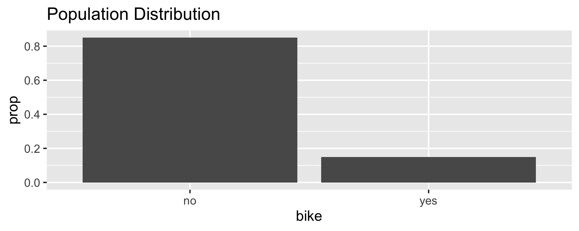
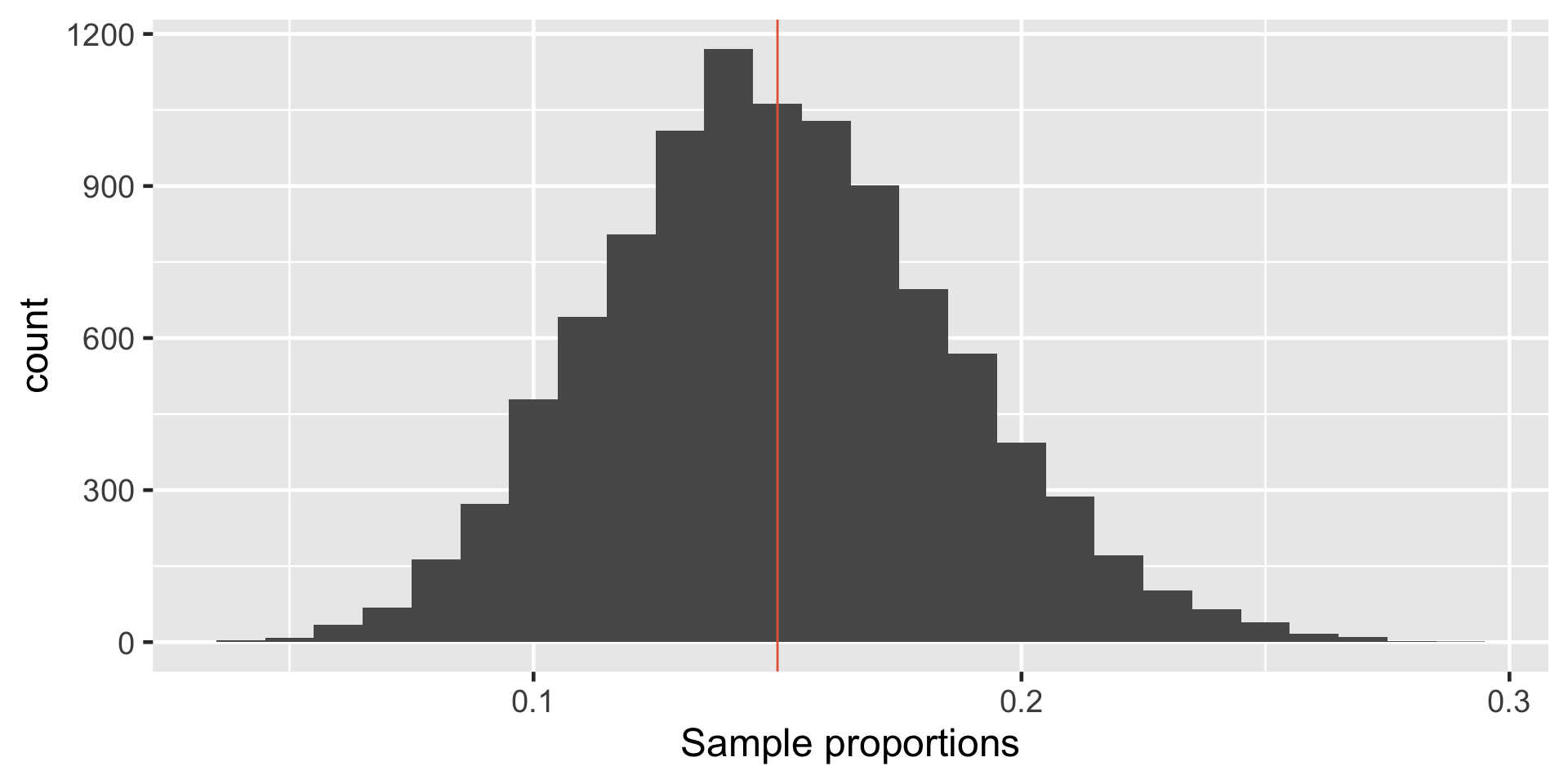
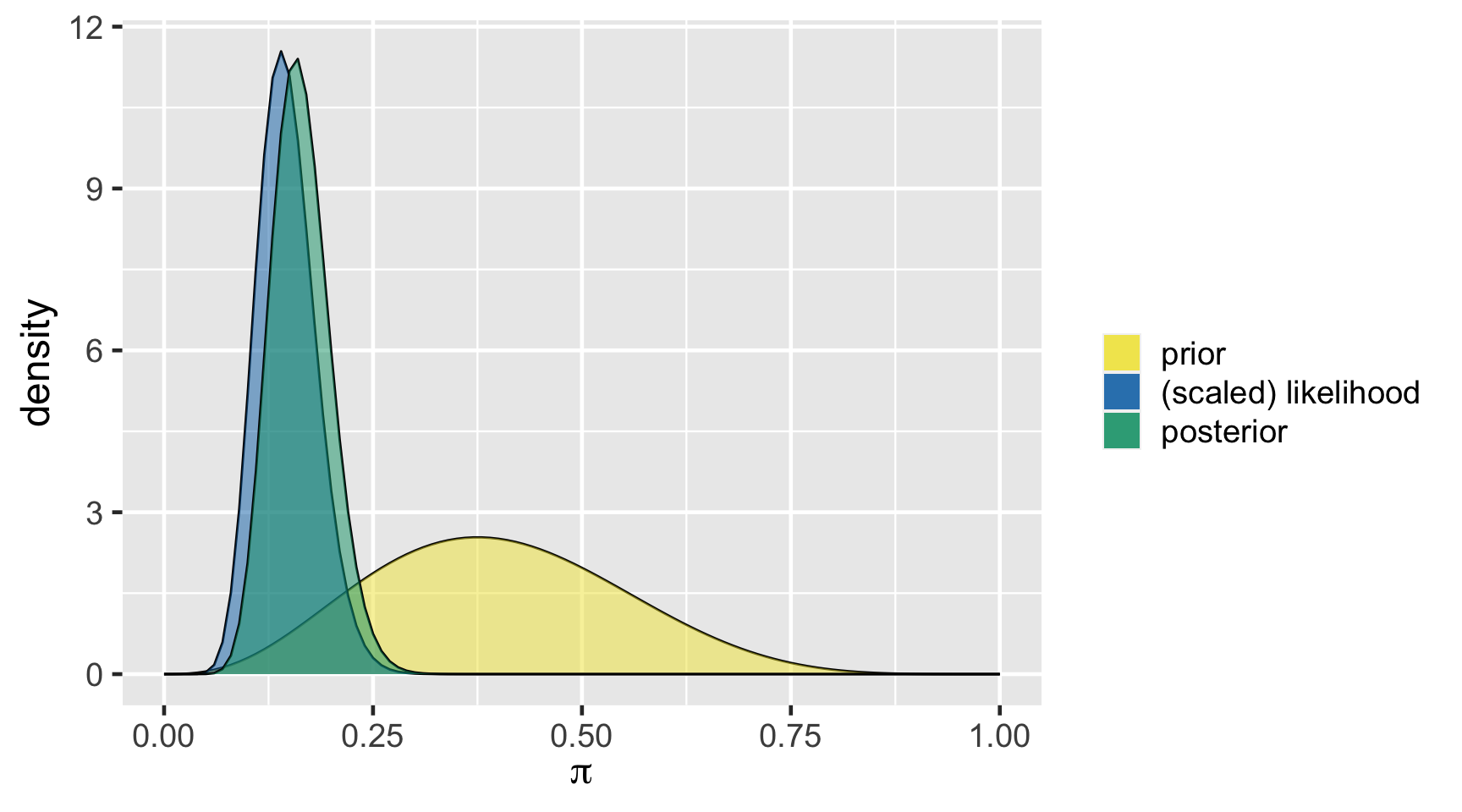
Let \(\pi\) represent the proportion of bike owners on campus then \(\pi =\) 0.15.

Getting to sampling distribution of single proportion

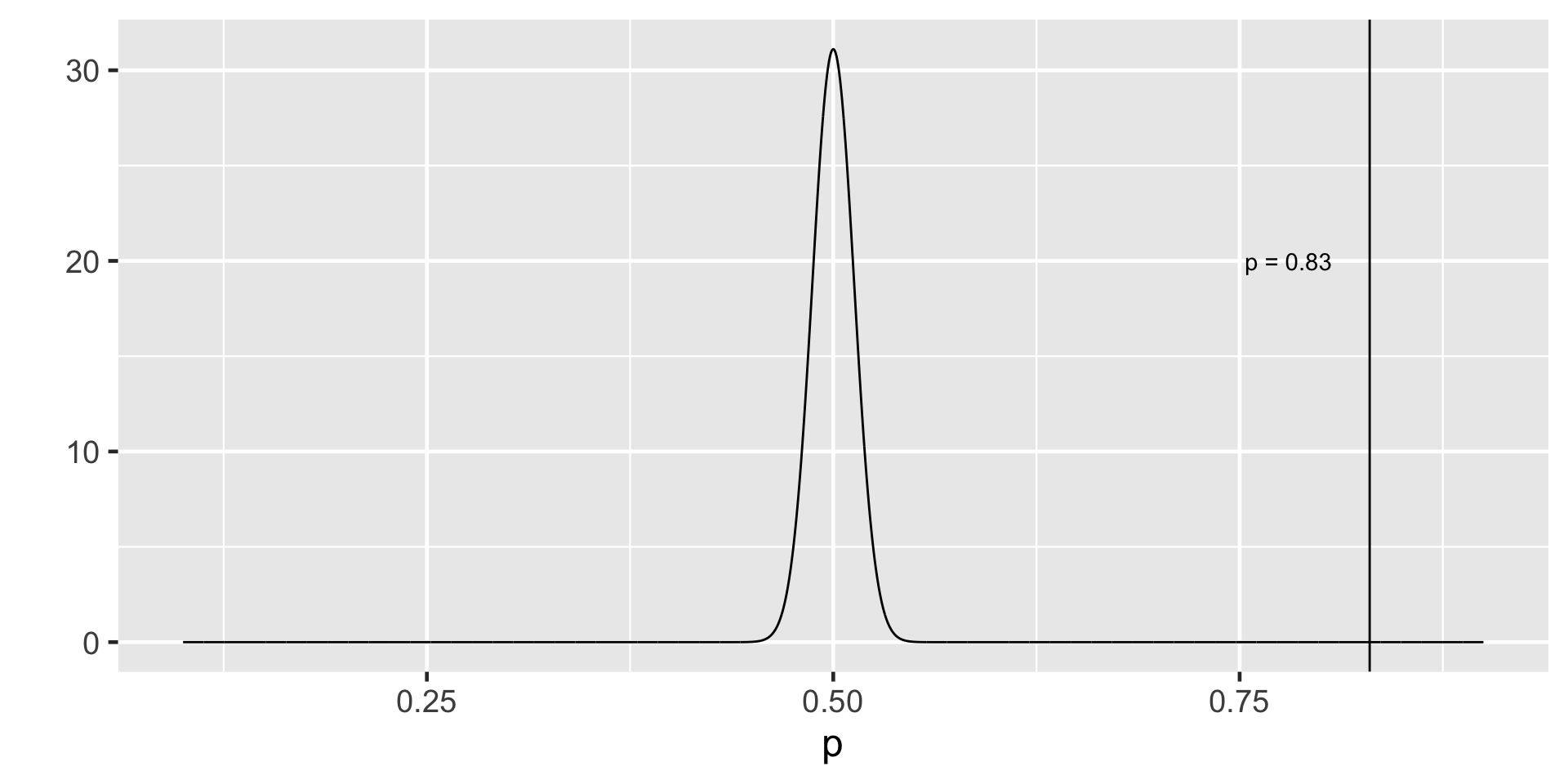
\(p_1\) - Proportion of first sample (n = 100)

[1] 0.17

\(p_2\) -Proportion of second sample (n = 100)

[1] 0.12

\(p_3\) -Proportion of third sample (n = 100)

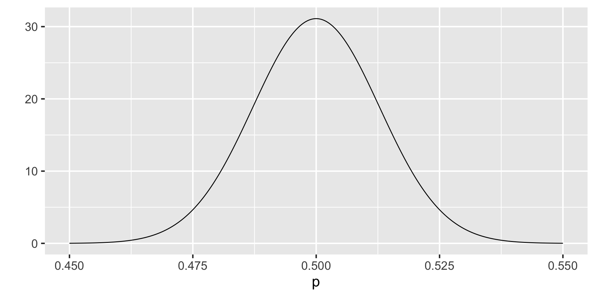
[1] 0.14

Sampling Distribution of Single Proportion

If certain conditions are met then

\[p \sim \text{approximately } N(\pi, \frac{\pi(1-\pi)}{n})\]

In Reality

• We only have one sample and thus one point estimate of the population parameter. How can make use of it?

• First we will assume the sample proportion is the best thing we have at hand and use it as a point estimate of the population proportion.

• Second, even though we embrace the sample proportion as a point estimate of the population proportion, we will need to acknowledge that it has some error.

Standard Error

\(p \sim \text{approximately } N(\text{mean} = \pi, \text{sd} = \sqrt{\frac{\pi(1-\pi)}{n}})\)

We call the standard deviation of the sampling distribution standard error of the estimate.

Standard error of single proportion is \(\sqrt{\frac{p(1-p)}{n}}\).

Confidence Interval

CI = \(\text{point estimate} \pm \text { margin of error}\)

CI = \(\text{point estimate} \pm \text { critical value} \times \text{standard error}\)

CI for single proportion = \(p \pm \text {critical value} \times \text{standard error}\)

CI for single proportion = \(p \pm \text {critical value} \times \sqrt{\frac{p(1-p)}{n}}\)

95% CI for single proportion = \(p \pm 1.96 \times \sqrt{\frac{p(1-p)}{n}}\) because …

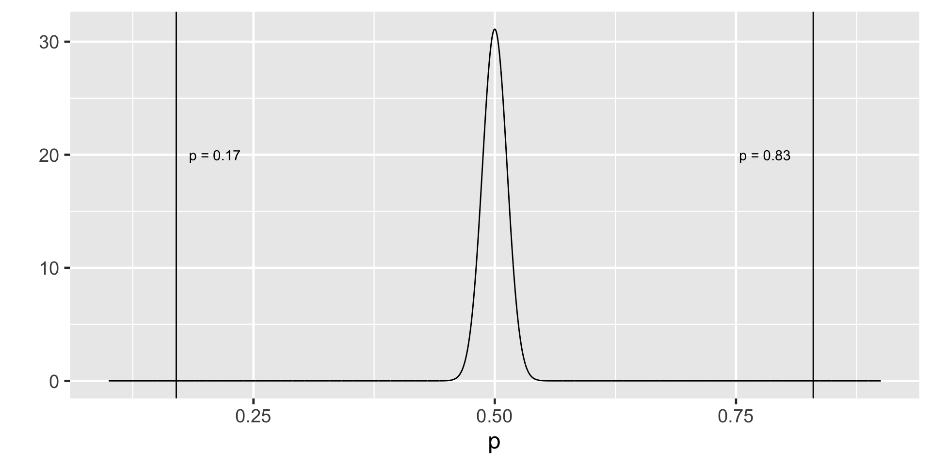
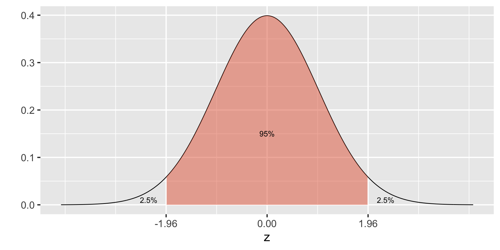
95% of the data falls within 1.96 standard deviations in the normal distribution.

How do we know that?

qnorm(0.025, mean = 0 , sd = 1)

[1] -1.959964

qnorm(0.975, mean = 0 , sd = 1)

[1] 1.959964

95% CI for the first sample

Recall \(p = 0.17\) and \(n = 100\)

95% CI for single proportion = \(p \pm 1.96 \times \sqrt{\frac{p(1-p)}{n}}\)

95% CI = \(0.17 \pm 1.96 \times \sqrt{\frac{0.17(1-0.17)}{100}}\)

95% CI = \(0.17 \pm 1.96 \times 0.03756328\)

95%CI = \(0.17 \pm 0.07362403\)

95%CI = (0.09637597, 0.243624)

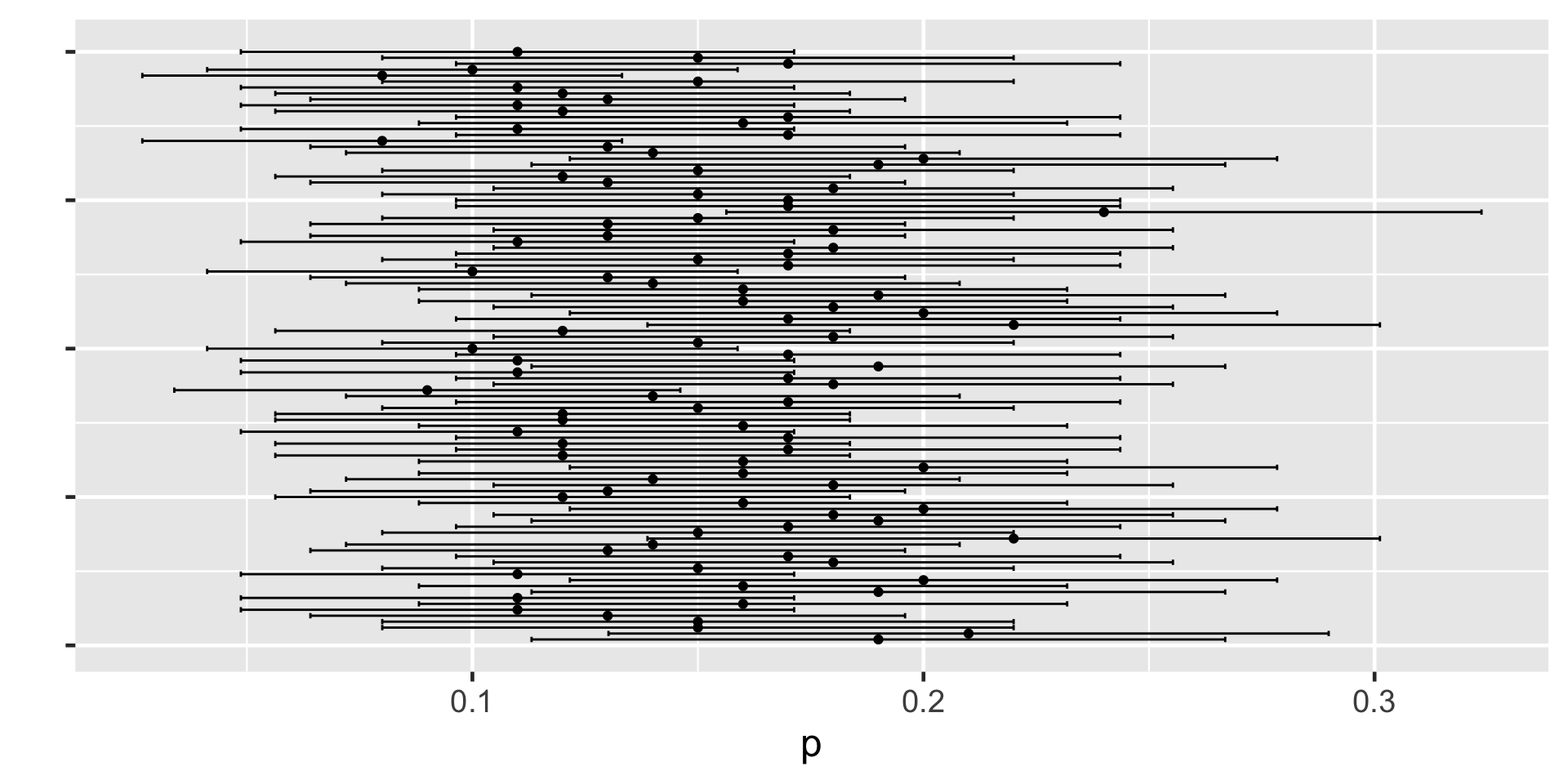
95% CI for the first sample

95%CI = (0.09637597, 0.243624)

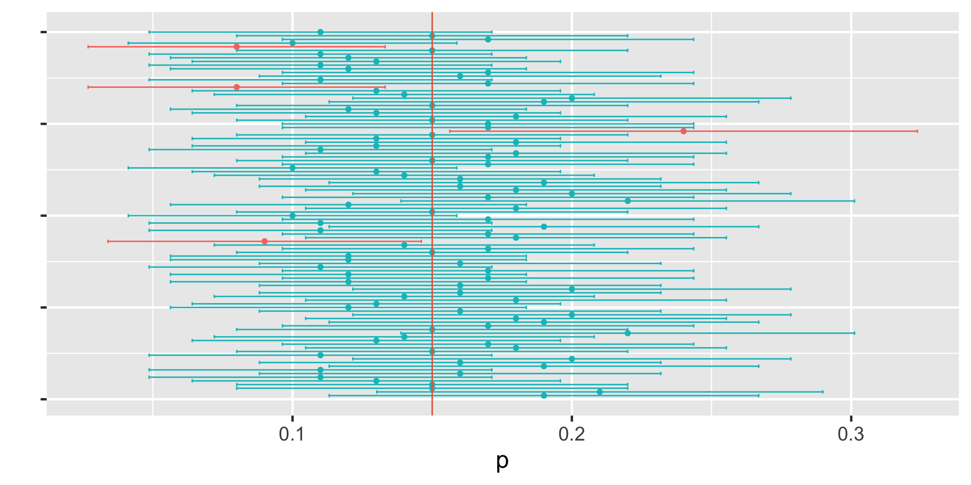
We are 95% confident that the true population proportion of bike owners is in this confidence interval.

class: middle center

95%CI = (0.09637597, 0.243624)

Understanding Confidence Intervals

I have taken 100 samples with \(n = 100\), calculated the sample proportion, standard error, and 95% CI interval for each sample

# A tibble: 100 × 4
       p     SE lower_bound upper_bound
   <dbl>  <dbl>       <dbl>       <dbl>
 1  0.19 0.0392      0.113        0.267
 2  0.21 0.0407      0.130        0.290
 3  0.15 0.0357      0.0800       0.220
 4  0.15 0.0357      0.0800       0.220
 5  0.13 0.0336      0.0641       0.196
 6  0.11 0.0313      0.0487       0.171
 7  0.16 0.0367      0.0881       0.232
 8  0.11 0.0313      0.0487       0.171
 9  0.19 0.0392      0.113        0.267
10  0.16 0.0367      0.0881       0.232
# ℹ 90 more rows

Understanding Confidence Intervals

Understanding Confidence Intervals

• The confidence interval can be expressed in terms of a long-run frequency in repeated samples (or in resampling): “Were this procedure to be repeated on numerous samples, the proportion of calculated 95% confidence intervals that encompassed the true value of the population parameter would tend toward 95%.”

• The confidence interval can be expressed in terms of probability with respect to a single theoretical (yet to be realized) sample: “There is a 95% probability that the 95% confidence interval calculated from a given future sample will cover the true value of the population parameter.” This essentially reframes the “repeated samples” interpretation as a probability rather than a frequency.

• The confidence interval can be expressed in terms of statistical significance, e.g.: “The 95% confidence interval represents values that are not statistically significantly different from the point estimate at the .05 level.”

Bayesian Inference

library(bayesrules)
data(moma_sample)
glimpse(moma_sample)

Rows: 100
Columns: 10
$ artist            <fct> Ad Gerritsen, Kirstine Roepstorff, Lisa Baumgardner,…
$ country           <fct> dutch, danish, american, american, american, canadia…
$ birth             <fct> 1940, 1972, 1958, 1952, 1946, 1927, 1901, 1941, 1920…
$ death             <fct> 2015, NA, 2015, NA, NA, 1966, 1971, NA, 2007, NA, NA…
$ alive             <lgl> FALSE, TRUE, FALSE, TRUE, TRUE, FALSE, FALSE, TRUE, …
$ genx              <lgl> FALSE, TRUE, FALSE, FALSE, FALSE, FALSE, FALSE, FALS…
$ gender            <fct> male, female, female, male, male, male, male, male, …
$ count             <int> 1, 3, 2, 1, 1, 8, 2, 1, 1, 5, 1, 2, 1, 1, 21, 16, 1,…
$ year_acquired_min <fct> 1981, 2005, 2016, 2001, 2012, 2008, 2018, 1981, 1949…
$ year_acquired_max <fct> 1981, 2005, 2016, 2001, 2012, 2008, 2018, 1981, 1949…

\[Y|\pi \sim \text{Bin}(100, \pi)\]

\[\pi \sim \text{Beta}(4, 6)\]

moma_sample %>% 
  mutate(genx = (birth >= 1965)) %>% 
  janitor::tabyl(genx)

 genx   n percent valid_percent
   NA 100       1            NA

\[\begin{split} Y | \pi & \sim \text{Bin}(100, \pi) \\ \pi & \sim \text{Beta}(4, 6) \\ \end{split} \;\;\;\; \Rightarrow \;\;\;\; \pi | (Y = 14) \sim \text{Beta}(18, 92)\]

plot_beta_binomial(alpha = 4, beta = 6, y = 14, n = 100)

summarize_beta_binomial(4, 6, y = 14, n = 100)

      model alpha beta      mean      mode         var         sd
1     prior     4    6 0.4000000 0.3750000 0.021818182 0.14770979
2 posterior    18   92 0.1636364 0.1574074 0.001232969 0.03511365

95% Posterior Credible Interval (CI)

0.025th & 0.975th quantiles of the Beta(18,92) posterior

qbeta(c(0.025, 0.975), 18, 92)

[1] 0.1009084 0.2379286

\(\int_{0.1}^{0.24} f(\pi|(y=14)) d\pi \; \approx \; 0.95\)

\[\begin{split} H_0: & \; \; \pi \ge 0.20 \\ H_a: & \; \; \pi < 0.20 \\ \end{split}\]

# Posterior probability that pi < 0.20
post_prob <- pbeta(0.20, 18, 92)
post_prob

[1] 0.8489856

\[\text{Posterior odds } = \frac{P(H_a \; | \; (Y=14))}{P(H_0 \; | \; (Y=14))} \approx 5.62 \]

# Posterior odds
post_odds <- post_prob / (1 - post_prob)
post_odds

[1] 5.621883

\[P(\pi<0.20)\]

prior_prob <- pbeta(0.20, 4, 6)
prior_prob

[1] 0.08564173

\[\text{Prior odds } = \frac{P(H_a)}{P(H_0)} \approx 0.093 \; .\]

prior_odds <- prior_prob / (1 - prior_prob)
prior_odds

[1] 0.09366321

The Bayes Factor (BF) compares the posterior odds to the prior odds, hence provides insight into just how much our understanding about Gen X representation evolved upon observing our sample data:

\[\text{Bayes Factor} = \frac{\text{Posterior odds }}{\text{Prior odds }}\]

Bayes Factor

In a hypothesis test of two competing hypotheses, \(H_a\) vs \(H_0\), the Bayes Factor is an odds ratio for \(H_a\):

\[\text{Bayes Factor} = \frac{\text{Posterior odds}}{\text{Prior odds}} = \frac{P(H_a | Y) / P(H_0 | Y)}{P(H_a) / P(H_0)} \; .\]

As a ratio, it’s meaningful to compare the Bayes Factor (BF) to 1. To this end, consider three possible scenarios:

1. BF = 1: The plausibility of \(H_a\) didn’t change in light of the observed data.
2. BF > 1: The plausibility of \(H_a\) increased in light of the observed data. Thus the greater the Bayes Factor, the more convincing the evidence for \(H_a\).
3. BF < 1: The plausibility of \(H_a\) decreased in light of the observed data.

Two-sided Tests

\[\begin{split} H_0: & \; \; \pi = 0.3 \\ H_a: & \; \; \pi \ne 0.3 \\ \end{split}\]

\[\text{Posterior odds } = \frac{P(H_a \; | \; (Y=14))}{P(H_0 \; | \; (Y=14))} = \frac{1}{0} = \text{ nooooo!}\]

Recall 95% posterior CI

[1] 0.1009084 0.2379286

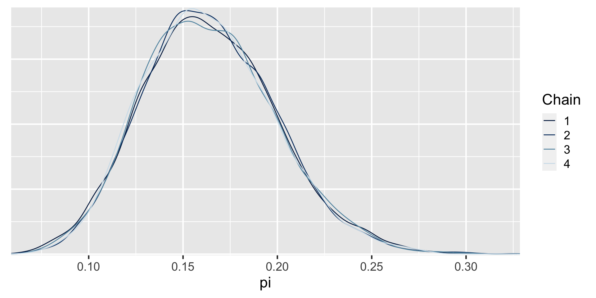
SAMPLING FOR MODEL '40889b2266edb1362fe73358abd137b3' NOW (CHAIN 1).
Chain 1: 
Chain 1: Gradient evaluation took 2.1e-05 seconds
Chain 1: 1000 transitions using 10 leapfrog steps per transition would take 0.21 seconds.
Chain 1: Adjust your expectations accordingly!
Chain 1: 
Chain 1: 
Chain 1: Iteration:    1 / 10000 [  0%]  (Warmup)
Chain 1: Iteration: 1000 / 10000 [ 10%]  (Warmup)
Chain 1: Iteration: 2000 / 10000 [ 20%]  (Warmup)
Chain 1: Iteration: 3000 / 10000 [ 30%]  (Warmup)
Chain 1: Iteration: 4000 / 10000 [ 40%]  (Warmup)
Chain 1: Iteration: 5000 / 10000 [ 50%]  (Warmup)
Chain 1: Iteration: 5001 / 10000 [ 50%]  (Sampling)
Chain 1: Iteration: 6000 / 10000 [ 60%]  (Sampling)
Chain 1: Iteration: 7000 / 10000 [ 70%]  (Sampling)
Chain 1: Iteration: 8000 / 10000 [ 80%]  (Sampling)
Chain 1: Iteration: 9000 / 10000 [ 90%]  (Sampling)
Chain 1: Iteration: 10000 / 10000 [100%]  (Sampling)
Chain 1: 
Chain 1:  Elapsed Time: 0.017894 seconds (Warm-up)
Chain 1:                0.018165 seconds (Sampling)
Chain 1:                0.036059 seconds (Total)
Chain 1: 

SAMPLING FOR MODEL '40889b2266edb1362fe73358abd137b3' NOW (CHAIN 2).
Chain 2: 
Chain 2: Gradient evaluation took 1e-06 seconds
Chain 2: 1000 transitions using 10 leapfrog steps per transition would take 0.01 seconds.
Chain 2: Adjust your expectations accordingly!
Chain 2: 
Chain 2: 
Chain 2: Iteration:    1 / 10000 [  0%]  (Warmup)
Chain 2: Iteration: 1000 / 10000 [ 10%]  (Warmup)
Chain 2: Iteration: 2000 / 10000 [ 20%]  (Warmup)
Chain 2: Iteration: 3000 / 10000 [ 30%]  (Warmup)
Chain 2: Iteration: 4000 / 10000 [ 40%]  (Warmup)
Chain 2: Iteration: 5000 / 10000 [ 50%]  (Warmup)
Chain 2: Iteration: 5001 / 10000 [ 50%]  (Sampling)
Chain 2: Iteration: 6000 / 10000 [ 60%]  (Sampling)
Chain 2: Iteration: 7000 / 10000 [ 70%]  (Sampling)
Chain 2: Iteration: 8000 / 10000 [ 80%]  (Sampling)
Chain 2: Iteration: 9000 / 10000 [ 90%]  (Sampling)
Chain 2: Iteration: 10000 / 10000 [100%]  (Sampling)
Chain 2: 
Chain 2:  Elapsed Time: 0.018052 seconds (Warm-up)
Chain 2:                0.019912 seconds (Sampling)
Chain 2:                0.037964 seconds (Total)
Chain 2: 

SAMPLING FOR MODEL '40889b2266edb1362fe73358abd137b3' NOW (CHAIN 3).
Chain 3: 
Chain 3: Gradient evaluation took 2e-06 seconds
Chain 3: 1000 transitions using 10 leapfrog steps per transition would take 0.02 seconds.
Chain 3: Adjust your expectations accordingly!
Chain 3: 
Chain 3: 
Chain 3: Iteration:    1 / 10000 [  0%]  (Warmup)
Chain 3: Iteration: 1000 / 10000 [ 10%]  (Warmup)
Chain 3: Iteration: 2000 / 10000 [ 20%]  (Warmup)
Chain 3: Iteration: 3000 / 10000 [ 30%]  (Warmup)
Chain 3: Iteration: 4000 / 10000 [ 40%]  (Warmup)
Chain 3: Iteration: 5000 / 10000 [ 50%]  (Warmup)
Chain 3: Iteration: 5001 / 10000 [ 50%]  (Sampling)
Chain 3: Iteration: 6000 / 10000 [ 60%]  (Sampling)
Chain 3: Iteration: 7000 / 10000 [ 70%]  (Sampling)
Chain 3: Iteration: 8000 / 10000 [ 80%]  (Sampling)
Chain 3: Iteration: 9000 / 10000 [ 90%]  (Sampling)
Chain 3: Iteration: 10000 / 10000 [100%]  (Sampling)
Chain 3: 
Chain 3:  Elapsed Time: 0.017845 seconds (Warm-up)
Chain 3:                0.018493 seconds (Sampling)
Chain 3:                0.036338 seconds (Total)
Chain 3: 

SAMPLING FOR MODEL '40889b2266edb1362fe73358abd137b3' NOW (CHAIN 4).
Chain 4: 
Chain 4: Gradient evaluation took 2e-06 seconds
Chain 4: 1000 transitions using 10 leapfrog steps per transition would take 0.02 seconds.
Chain 4: Adjust your expectations accordingly!
Chain 4: 
Chain 4: 
Chain 4: Iteration:    1 / 10000 [  0%]  (Warmup)
Chain 4: Iteration: 1000 / 10000 [ 10%]  (Warmup)
Chain 4: Iteration: 2000 / 10000 [ 20%]  (Warmup)
Chain 4: Iteration: 3000 / 10000 [ 30%]  (Warmup)
Chain 4: Iteration: 4000 / 10000 [ 40%]  (Warmup)
Chain 4: Iteration: 5000 / 10000 [ 50%]  (Warmup)
Chain 4: Iteration: 5001 / 10000 [ 50%]  (Sampling)
Chain 4: Iteration: 6000 / 10000 [ 60%]  (Sampling)
Chain 4: Iteration: 7000 / 10000 [ 70%]  (Sampling)
Chain 4: Iteration: 8000 / 10000 [ 80%]  (Sampling)
Chain 4: Iteration: 9000 / 10000 [ 90%]  (Sampling)
Chain 4: Iteration: 10000 / 10000 [100%]  (Sampling)
Chain 4: 
Chain 4:  Elapsed Time: 0.018097 seconds (Warm-up)
Chain 4:                0.019304 seconds (Sampling)
Chain 4:                0.037401 seconds (Total)
Chain 4: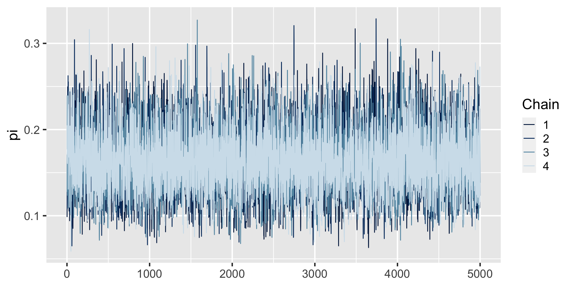 

library(bayesplot)
# Parallel trace plots & density plots
mcmc_trace(art_sim, pars = "pi", size = 0.5)

  post_mean post_mode  lower_95 upper_95
1 0.1640626 0.1528862 0.1006243 0.239346

 exceeds     n percent
   FALSE  3079 0.15395
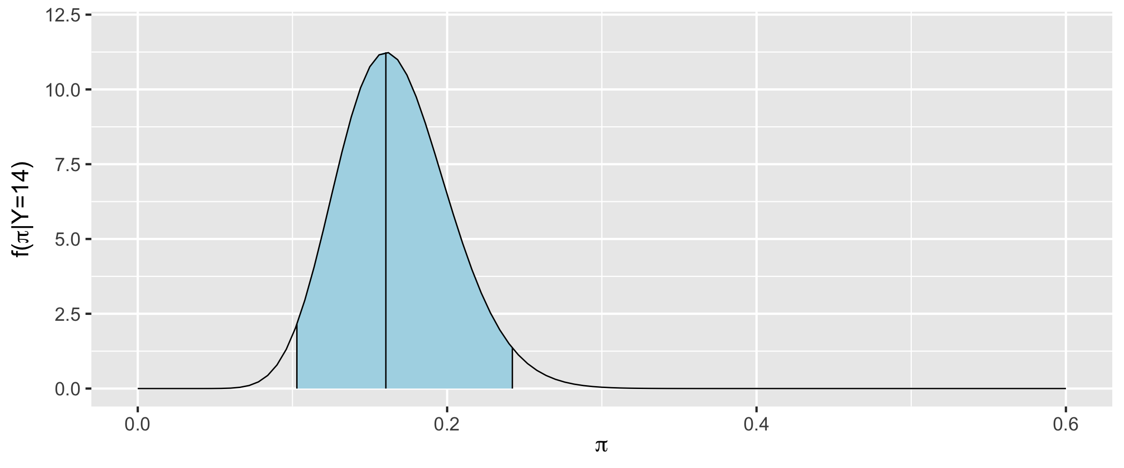
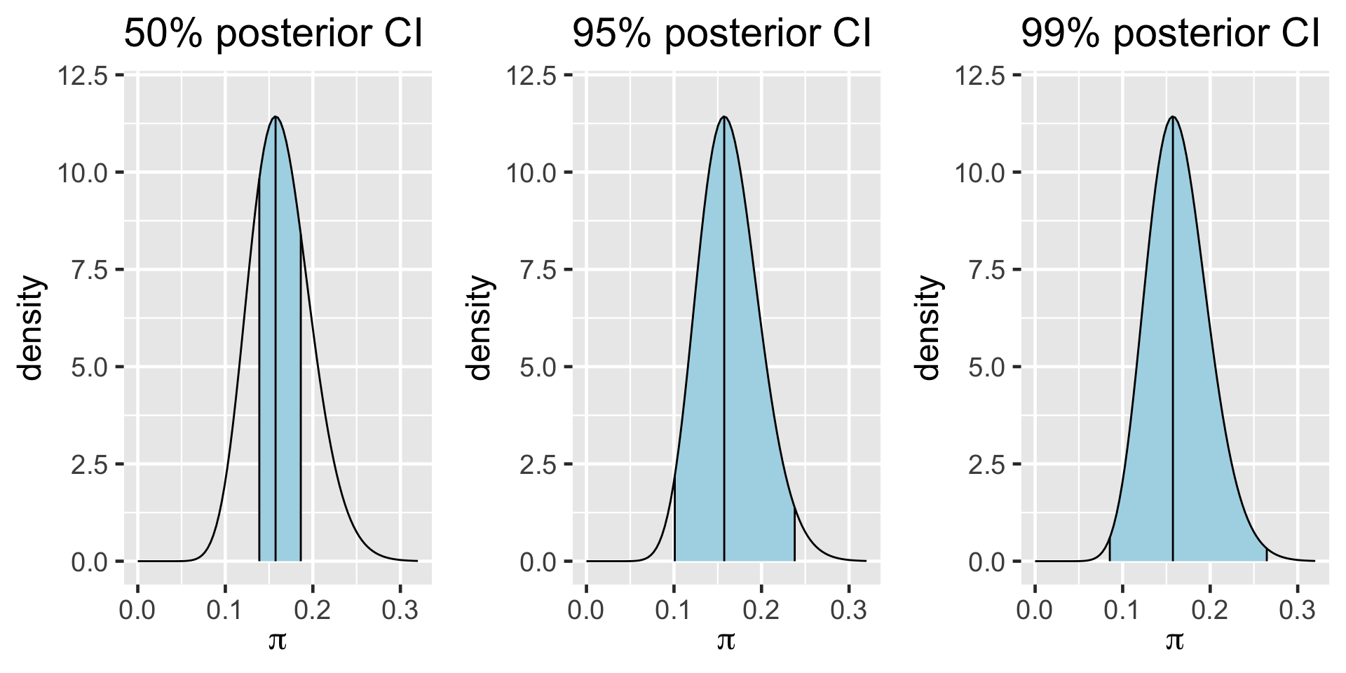
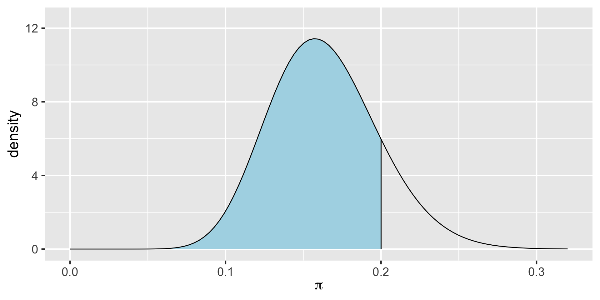
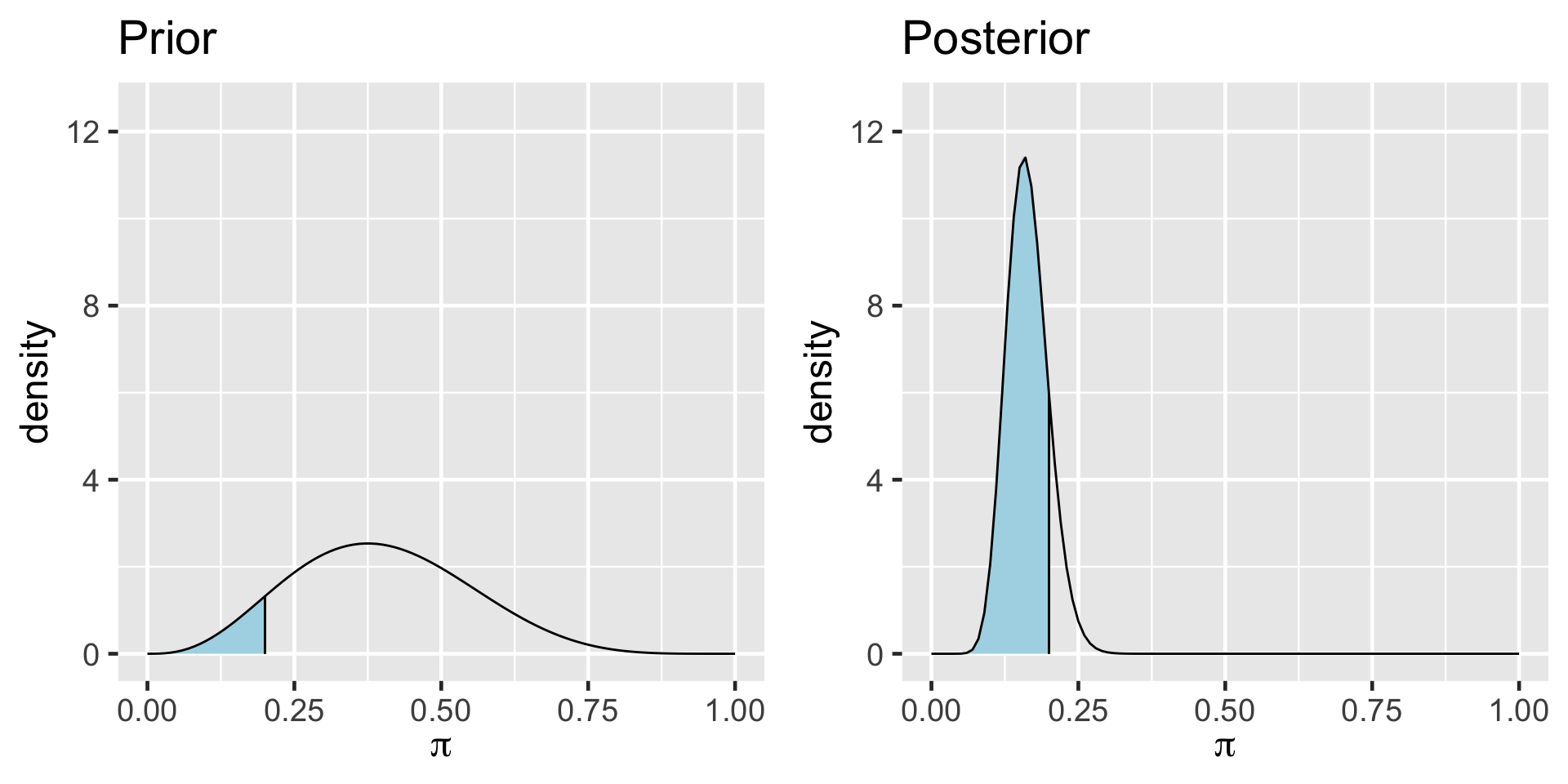
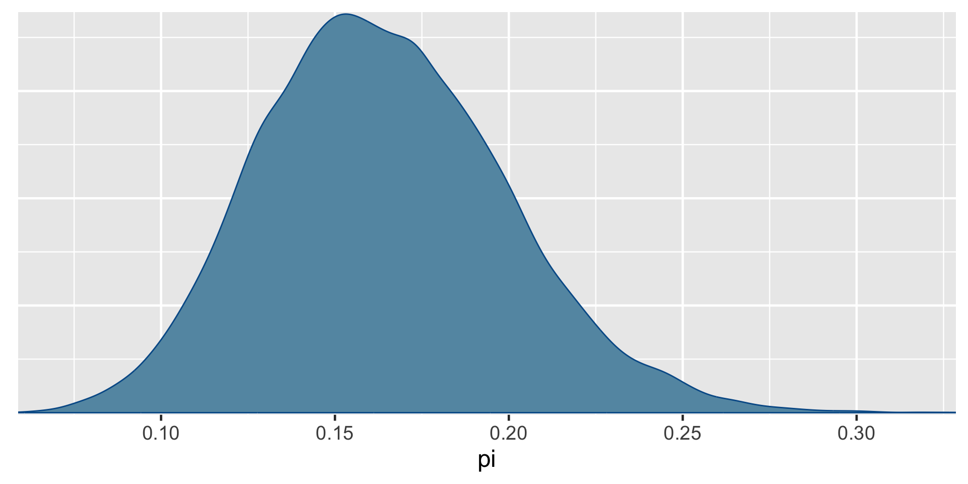
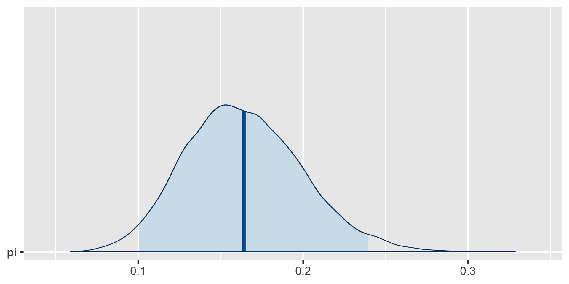
    TRUE 16921 0.84605

[1] 0.8489856

a Bayesian analysis assesses the uncertainty regarding an unknown parameter \(\pi\) in light of observed data \(Y\).

\[P((\pi < 0.20) \; | \; (Y = 14)) = 0.8489856 \;.\]

a frequentist analysis assesses the uncertainty of the observed data \(Y\) in light of assumed values of \(\pi\).

\[P((Y \le 14) | (\pi = 0.20)) = 0.08\]