Fitting regression models

Day 4

Note that examples in this lecture are a simplified version of Chapter 9 of Bayes Rules! book.

Packages

library(bayesrules)
library(tidyverse)
library(rstanarm)
library(bayesplot)
library(broom.mixed)
theme_set(theme_gray(base_size = 18)) # change default font size in ggplot

Data

glimpse(bikes)

Rows: 500
Columns: 13
$ date        <date> 2011-01-01, 2011-01-03, 2011-01-04, 2011-01-05, 2011-01-0…
$ season      <fct> winter, winter, winter, winter, winter, winter, winter, wi…
$ year        <int> 2011, 2011, 2011, 2011, 2011, 2011, 2011, 2011, 2011, 2011…
$ month       <fct> Jan, Jan, Jan, Jan, Jan, Jan, Jan, Jan, Jan, Jan, Jan, Jan…
$ day_of_week <fct> Sat, Mon, Tue, Wed, Fri, Sat, Mon, Tue, Wed, Thu, Fri, Sat…
$ weekend     <lgl> TRUE, FALSE, FALSE, FALSE, FALSE, TRUE, FALSE, FALSE, FALS…
$ holiday     <fct> no, no, no, no, no, no, no, no, no, no, no, no, no, yes, n…
$ temp_actual <dbl> 57.39952, 46.49166, 46.76000, 48.74943, 46.50332, 44.17700…
$ temp_feel   <dbl> 64.72625, 49.04645, 51.09098, 52.63430, 50.79551, 46.60286…
$ humidity    <dbl> 80.5833, 43.7273, 59.0435, 43.6957, 49.8696, 53.5833, 48.2…
$ windspeed   <dbl> 10.749882, 16.636703, 10.739832, 12.522300, 11.304642, 17.…
$ weather_cat <fct> categ2, categ1, categ1, categ1, categ2, categ2, categ1, ca…
$ rides       <int> 654, 1229, 1454, 1518, 1362, 891, 1280, 1220, 1137, 1368, …

Rides

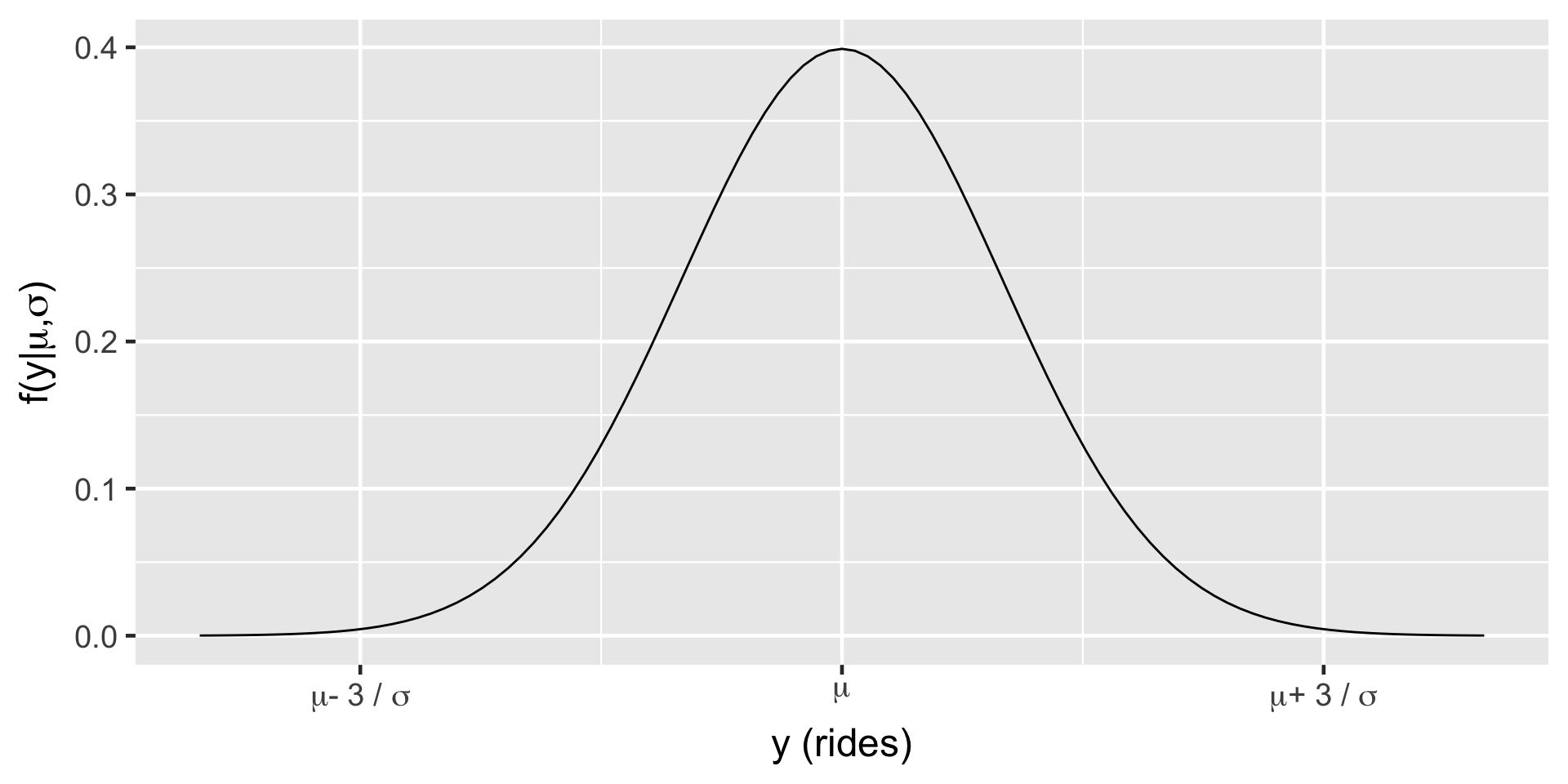
\(Y_i | \mu, \sigma \stackrel{ind}{\sim} N(\mu, \sigma^2)\)
\(\mu \sim N(\theta, \tau^2)\) \(\sigma \sim \text{ some prior model.}\)

Regression Model

\(Y_i\) the number of rides
\(X_i\) temperature (in Fahrenheit) on day \(i\).

\(\mu_i = \beta_0 + \beta_1X_i\)

\(\beta_0:\) the typical ridership on days in which the temperature was 0 degrees ( \(X_i\)=0). It is not interpretable in this case.

\(\beta_1:\) the typical change in ridership for every one unit increase in temperature.

Normal likelihood model

\[\begin{split} Y_i | \beta_0, \beta_1, \sigma & \stackrel{ind}{\sim} N\left(\mu_i, \sigma^2\right) \;\; \text{ with } \;\; \mu_i = \beta_0 + \beta_1X_i \; .\\ \end{split}\]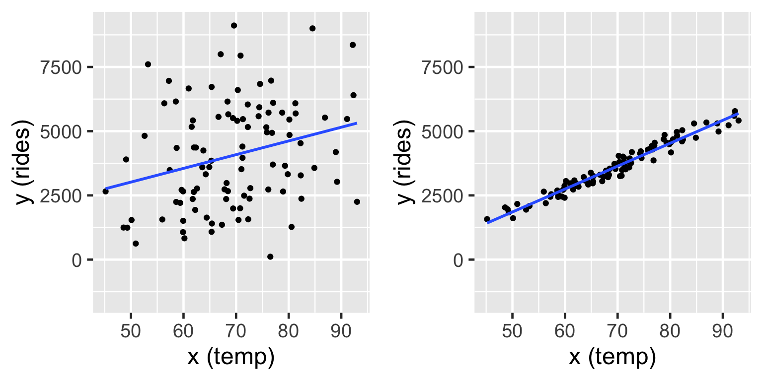

From previous slide

Both the model lines show cases where \(\beta_0 = -2000\) and slope \(\beta_1 = 100\). On the left \(\sigma = 2000\) and on the right \(\sigma = 200\) (right). In both cases, the model line is defined by \(\beta_0 + \beta_1 x = -2000 + 100 x\).

Model

\(\text{likelihood:} \; \; \; Y_i | \beta_0, \beta_1, \sigma \;\;\;\stackrel{ind}{\sim} N\left(\mu_i, \sigma^2\right)\text{ with } \mu_i = \beta_0 + \beta_1X_i\)

\(\text{prior models:}\)

\(\beta_0\sim N(m_0, s_0^2 )\)
\(\beta_1\sim N(m_1, s_1^2 )\)
\(\sigma \sim \text{Exp}(l)\)

Note:

\(\text{Exp}(l) = \text{Gamma}(1, l)\)

Model building: One step at a time

Let \(Y\) be a response variable and \(X\) be a predictor or set of predictors. Then we can build a model of \(Y\) by \(X\) through the following general principles:

• Take note of whether \(Y\) is discrete or continuous. Accordingly, identify an appropriate model structure of data \(Y\) (e.g., Normal, Poisson, Binomial).
• Rewrite the mean of \(Y\) as a function of predictors \(X\) (e.g., \(\mu = \beta_0 + \beta_1 X\)).
• Identify all unknown model parameters in your model (e.g., \(\beta_0, \beta_1, \sigma\)).
• Take note of the values that each of these parameters might take. Accordingly, identify appropriate prior models for these parameters.

Suppose we have the following prior understanding of this relationship:

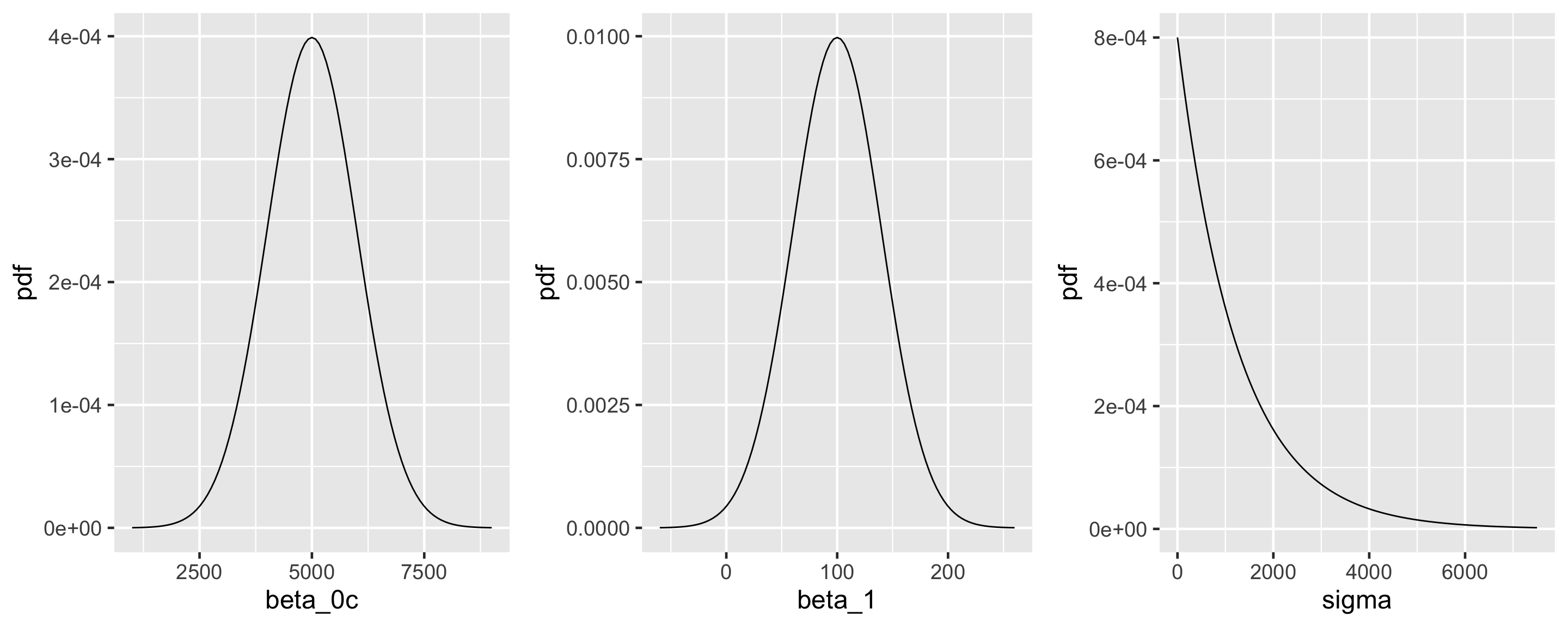
1. On an average temperature day, say 65 or 70 degrees for D.C., there are typically around 5000 riders, though this average could be somewhere between 3000 and 7000.

2. For every one degree increase in temperature, ridership typically increases by 100 rides, though this average increase could be as low as 20 or as high as 180.

3. At any given temperature, daily ridership will tend to vary with a moderate standard deviation of 1250 rides.

plot_normal(mean = 5000, sd = 1000) + 
  labs(x = "beta_0c", y = "pdf")

plot_normal(mean = 100, sd = 40) + 
  labs(x = "beta_1", y = "pdf")

plot_gamma(shape = 1, rate = 0.0008) + 
  labs(x = "sigma", y = "pdf")

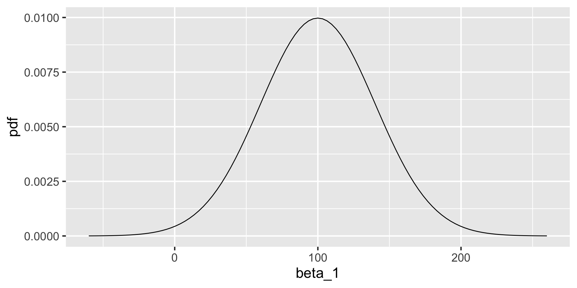
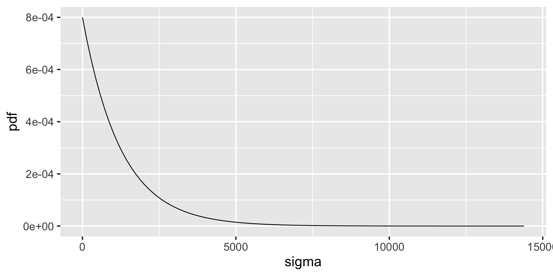
\[\begin{split} Y_i | \beta_0, \beta_1, \sigma & \stackrel{ind}{\sim} N\left(\mu_i, \sigma^2\right) \;\; \text{ with } \;\; \mu_i = \beta_0 + \beta_1X_i \\ \beta_{0c} & \sim N\left(5000, 1000^2 \right) \\ \beta_1 & \sim N\left(100, 40^2 \right) \\ \sigma & \sim \text{Exp}(0.0008) .\\ \end{split}\]

Simulation via rstanarm

#|cache: true
bike_model <- stan_glm(rides ~ temp_feel, data = bikes,
                       family = gaussian,
                       prior_intercept = normal(5000, 1000),
                       prior = normal(100, 40), 
                       prior_aux = exponential(0.0008),
                       chains = 4, iter = 5000*2, seed = 84735,
                       refresh = FALSE) 

The refresh = FALSE prevents printing out your chains and iterations, especially useful in Quarto.

# Effective sample size ratio and Rhat
neff_ratio(bike_model)

(Intercept)   temp_feel       sigma 
    1.03285     1.03505     0.96585 

rhat(bike_model)

(Intercept)   temp_feel       sigma 
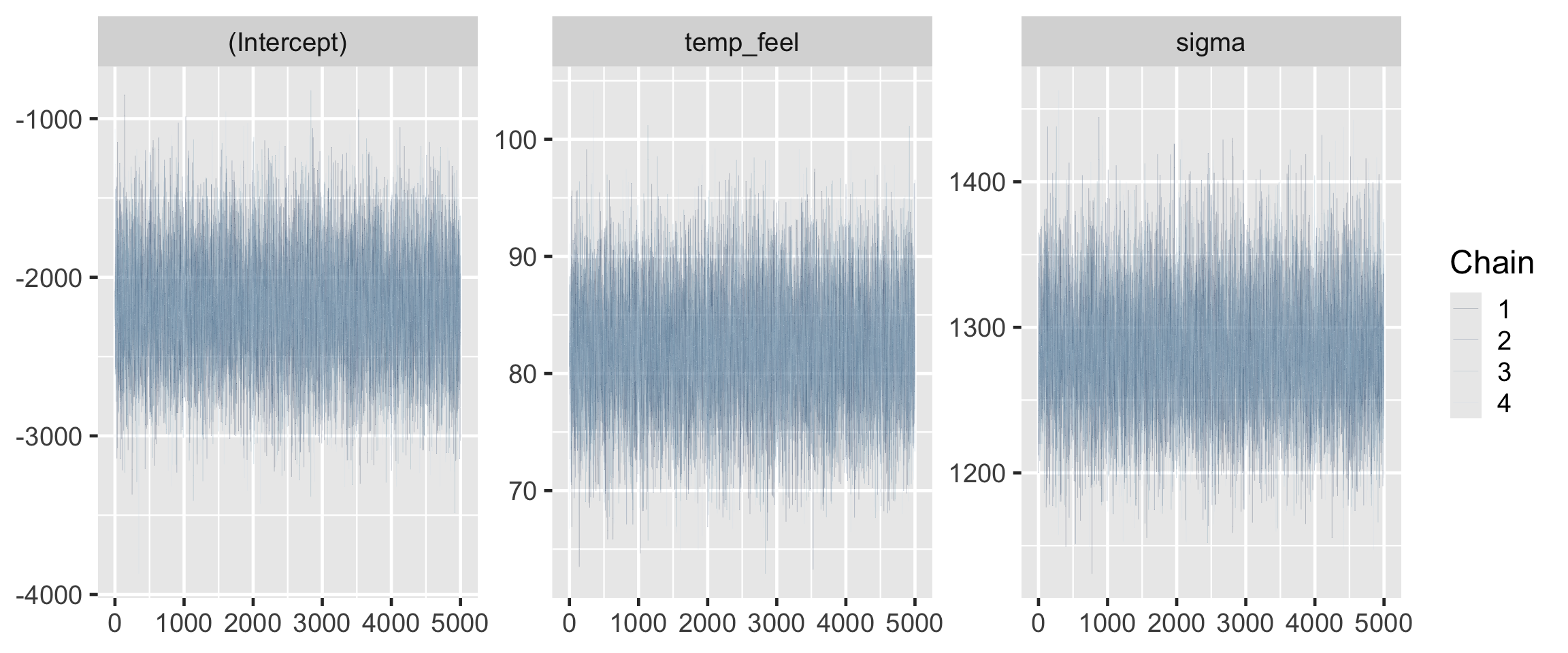
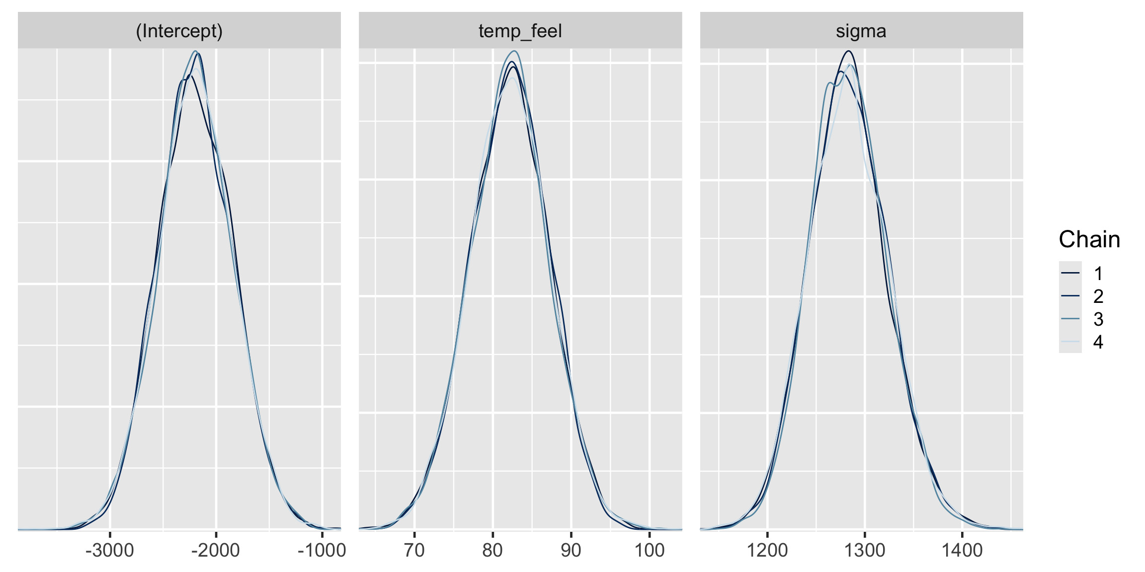
  0.9998873   0.9999032   0.9999642 

The effective sample size ratios are slightly above 1 and the R-hat values are very close to 1, indicating that the chains are stable, mixing quickly, and behaving much like an independent sample.

mcmc_trace(bike_model, size = 0.1)

mcmc_dens_overlay(bike_model)

Simulation via rstan

# STEP 1: DEFINE the model
stan_bike_model <- "
  data {
    int<lower = 0> n;
    vector[n] Y;
    vector[n] X;
  }
  parameters {
    real beta0;
    real beta1;
    real<lower = 0> sigma;
  }
  model {
    Y ~ normal(beta0 + beta1 * X, sigma);
    beta0 ~ normal(-2000, 1000);
    beta1 ~ normal(100, 40);
    sigma ~ exponential(0.0008);
  }
"

Simulation via rstan

# STEP 2: SIMULATE the posterior
stan_bike_sim <- 
  stan(model_code = stan_bike_model, 
       data = list(n = nrow(bikes), Y = bikes$rides, X = bikes$temp_feel), 
       chains = 4, iter = 5000*2, seed = 84735)

Posterior summary statistics

tidy(bike_model, effects = c("fixed", "aux"),
     conf.int = TRUE, conf.level = 0.80)

# A tibble: 4 × 5
  term        estimate std.error conf.low conf.high
  <chr>          <dbl>     <dbl>    <dbl>     <dbl>
1 (Intercept)  -2195.     354.    -2646.    -1736. 
2 temp_feel       82.2      5.07     75.7      88.7
3 sigma         1282.      40.6    1232.     1336. 
4 mean_PPD      3487.      81.5    3382.     3593. 

The posterior median relationship is

\[\begin{equation} -2195.31 + 82.22 X. \end{equation}\]

# Store the 4 chains for each parameter in 1 data frame
bike_model_df <- as.data.frame(bike_model)

# Check it out
nrow(bike_model_df)

[1] 20000

head(bike_model_df, 3)

  (Intercept) temp_feel    sigma
1   -2125.091  80.92653 1230.511
2   -2087.977  80.60855 1200.141
3   -2265.712  83.64980 1365.039

# 50 simulated model lines
bikes %>%
  tidybayes::add_fitted_draws(bike_model, n = 50) %>%
  ggplot(aes(x = temp_feel, y = rides)) +
    geom_line(aes(y = .value, group = .draw), alpha = 0.15) + 
    geom_point(data = bikes, size = 0.05)

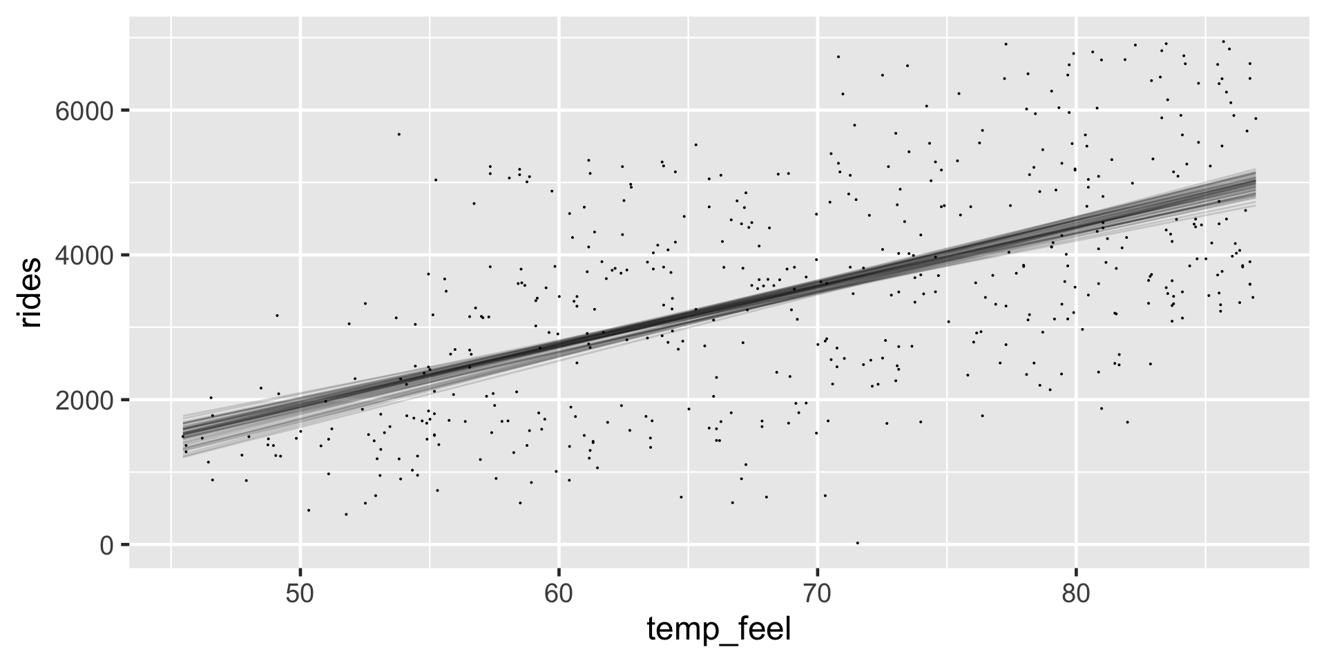
Do we have ample posterior evidence that there’s a positive association between ridership and temperature, i.e., that \(\beta_1 > 0\)?

Visual evidence In our visual examination of 50 posterior plausible scenarios for the relationship between ridership and temperature, all exhibited positive associations.

Numerical evidence from the posterior credible interval More rigorously, the 80% credible interval for \(\beta_1\) in tidy() summary, (75.7, 88.7), lies entirely and well above 0.

Numerical evidence from a posterior probability A quick tabulation approximates that there’s almost certainly a positive association, \(P(\beta_1 > 0 \; | \; \vec{y}) \approx 1\).

# Tabulate the beta_1 values that exceed 0
bike_model_df %>% 
  mutate(exceeds_0 = temp_feel > 0) %>% 
  janitor::tabyl(exceeds_0)

 exceeds_0     n percent
      TRUE 20000       1

Posterior prediction

Suppose a weather report indicates that tomorrow will be a 75-degree day in D.C. What’s your posterior guess of the number of riders that Capital Bikeshare should anticipate?

Do you think there will be 3971 riders tomorrow?

\[-2195.31 + 82.22*75 = 3971.19 .\]

There are two potential sources of variability:

• Sampling variability in the data
  The observed ridership outcomes, \(Y\), typically deviate from the model line. That is, we don’t expect every 75-degree day to have the same exact number of rides.

• Posterior variability in parameters \((\beta_0, \beta_1, \sigma)\)
  The posterior median model is merely the center in a range of plausible model lines \(\beta_0 + \beta_1 X\). We should consider this entire range as well as that in \(\sigma\), the degree to which observations might deviate from the model lines.

Posterior Predictive Model

Mathematically speaking:

\[f\left(y_{\text{new}} | \vec{y}\right) = \int\int\int f\left(y_{new} | \beta_0,\beta_1,\sigma\right) f(\beta_0,\beta_1,\sigma|\vec{y}) d\beta_0 d\beta_1 d\sigma .\]

Now, we don’t actually have a nice, tidy formula for the posterior pdf of our regression parameters, \(f(\beta_0,\beta_1,\sigma|\vec{y})\), and thus can’t get a nice tidy formula for the posterior predictive pdf \(f\left(y_{\text{new}} | \vec{y}\right)\). What we do have is 20,000 sets of parameters in the Markov chain \(\left(\beta_0^{(i)},\beta_1^{(i)},\sigma^{(i)}\right)\). We can then approximate the posterior predictive model for \(Y_{\text{new}}\) at \(X = 75\) by simulating a ridership prediction from the Normal model evaluated each parameter set:

\[Y_{\text{new}}^{(i)} | \beta_0, \beta_1, \sigma \; \sim \; N\left(\mu^{(i)}, \left(\sigma^{(i)}\right)^2\right) \;\; \text{ with } \;\; \mu^{(i)} = \beta_0^{(i)} + \beta_1^{(i)} \cdot 75.\]

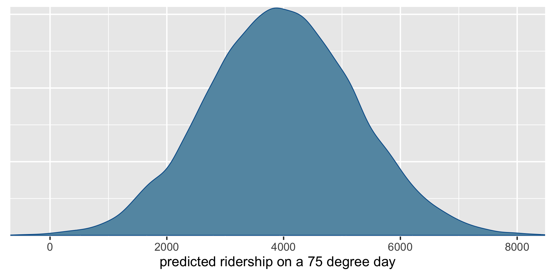
Thus, each of the 20,000 parameter sets in our Markov chain (left) produces a unique prediction (right):

\[\left[ \begin{array}{lll} \beta_0^{(1)} & \beta_1^{(1)} & \sigma^{(1)} \\ \beta_0^{(2)} & \beta_1^{(2)} & \sigma^{(2)} \\ \vdots & \vdots & \vdots \\ \beta_0^{(20000)} & \beta_1^{(20000)} & \sigma^{(20000)} \\ \end{array} \right] \;\; \longrightarrow \;\; \left[ \begin{array}{l} Y_{\text{new}}^{(1)} \\ Y_{\text{new}}^{(2)} \\ \vdots \\ Y_{\text{new}}^{(20000)} \\ \end{array} \right]\]

The resulting collection of 20,000 predictions, \(\left\lbrace Y_{\text{new}}^{(1)}, Y_{\text{new}}^{(2)}, \ldots, Y_{\text{new}}^{(20000)} \right\rbrace\), approximates the posterior predictive model of ridership \(Y\) on 75-degree days. We will obtain this approximation both “by hand,” which helps us build some powerful intuition, and using shortcut R functions.

Building a posterior predictive model

We’ll simulate 20,000 predictions of ridership on a 75-degree day, \(\left\lbrace Y_{\text{new}}^{(1)}, Y_{\text{new}}^{(2)}, \ldots, Y_{\text{new}}^{(20000)} \right\rbrace\), one from each parameter set in bike_model_df. Let’s start small with just the first posterior plausible parameter set:

first_set <- head(bike_model_df, 1)
first_set

  (Intercept) temp_feel    sigma
1   -2125.091  80.92653 1230.511

Under this particular scenario, \(\left(\beta_0^{(1)}, \beta_1^{(1)}, \sigma^{(1)}\right) = (-2125, 80.93, 1231)\), the average ridership at a given temperature is defined by

\[\mu = \beta_0^{(1)} + \beta_1^{(1)} X = -2125 + 80.93X .\]

As such, we’d expect an average of \(\mu = 3945\) riders on a 75-degree day:

mu <- first_set$`(Intercept)` + first_set$temp_feel * 75
mu

[1] 3944.398

To capture the sampling variability around this average, i.e., the fact that not all 75-degree days have the same ridership, we can simulate our first official prediction \(Y_{\text{new}}^{(1)}\) by taking a random draw from the Normal model specified by this first parameter set:

\[Y_{\text{new}}^{(1)} | \beta_0, \beta_1, \sigma \; \sim \; N\left(3944.75, 1231^2\right) .\]

Taking a draw from this model using rnorm(), we happen to observe an above average 4765 rides on the 75-degree day:

set.seed(84735)
y_new <- rnorm(1, mean = mu, sd = first_set$sigma)
y_new

[1] 4765.436

Now let’s do this 19,999 more times.

# Predict rides for each parameter set in the chain
set.seed(84735)
predict_75 <- bike_model_df %>% 
  mutate(mu = `(Intercept)` + temp_feel*75,
         y_new = rnorm(20000, mean = mu, sd = sigma))

head(predict_75, 3)

  (Intercept) temp_feel    sigma       mu    y_new
1   -2125.091  80.92653 1230.511 3944.398 4765.436
2   -2087.977  80.60855 1200.141 3957.664 3809.038
3   -2265.712  83.64980 1365.039 4008.023 5073.938

Whereas the collection of 20,000 mu values approximates the posterior model for the typical ridership on 75-degree days, \(\mu = \beta_0 + \beta_1 * 75\), the 20,000 y_new values approximate the posterior predictive model of ridership for tomorrow, an individual 75-degree day,

\[Y_{\text{new}} | \beta_0, \beta_1, \sigma \; \sim \; N\left(\mu, \sigma^2\right) \;\; \text{ with } \;\; \mu = \beta_0 + \beta_1 \cdot 75 .\]

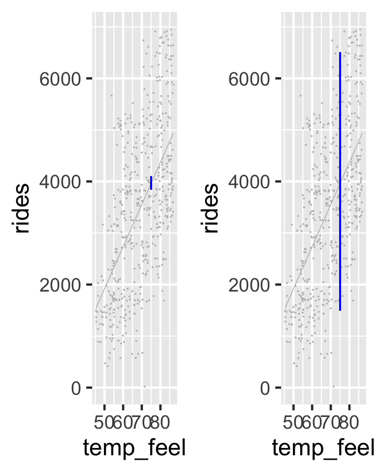
The 95% credible interval for the typical number of rides on a 75-degree day, \(\mu\), ranges from 3841 to 4097. In contrast, the 95% posterior prediction interval for the number of rides tomorrow has a much wider range from 1492 to 6503.

# Construct 95% posterior (predictive) credible intervals
predict_75 %>% 
  summarize(lower_mu = quantile(mu, 0.025),
            upper_mu = quantile(mu, 0.975),
            lower_new = quantile(y_new, 0.025),
            upper_new = quantile(y_new, 0.975))

  lower_mu upper_mu lower_new upper_new
1 3841.078 4096.946  1492.331  6502.669

# Plot the posterior model of the typical ridership on 75 degree days
ggplot(predict_75, aes(x = mu)) + 
  geom_density()

# Plot the posterior predictive model of tomorrow's ridership
ggplot(predict_75, aes(x = y_new)) + 
  geom_density()

The posterior model of \(\mu\), the typical ridership on a 75-degree day (left), and the posterior predictive model of the ridership tomorrow, a specific 75-degree day (right).

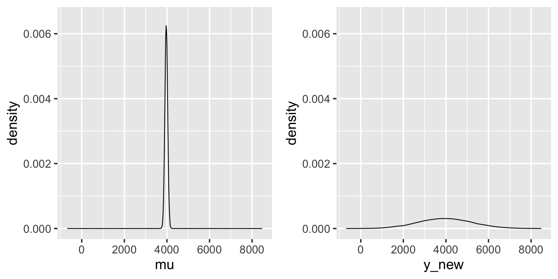
There’s more accuracy in anticipating the average behavior across multiple data points than the unique behavior of a single data point.

95% posterior credible intervals (blue) for the average ridership on 75-degree days (left) and the predicted ridership for tomorrow, an individual 75-degree day (right).

Posterior prediction with rstanarm

Simulating the posterior predictive model from scratch allowed you to really connect with the concept, but moving forward we can utilize the posterior_predict() function in the rstanarm package:

# Simulate a set of predictions
set.seed(84735)
shortcut_prediction <- 
  posterior_predict(bike_model, newdata = data.frame(temp_feel = 75))

The shortcut_prediction object contains 20,000 predictions of ridership on 75-degree days. We can both visualize and summarize the corresponding (approximate) posterior predictive model using our usual tricks. The results are equivalent to those we constructed from scratch above:

# Construct a 95% posterior credible interval
posterior_interval(shortcut_prediction, prob = 0.95)

      2.5%    97.5%
1 1492.331 6502.669

# Plot the approximate predictive model
mcmc_dens(shortcut_prediction) + 
  xlab("predicted ridership on a 75 degree day")

Posterior predictive model of ridership on a 75-degree day.