Discrete Response Data

Day 1

Note that this lecture is based on Chapters 3-4 of Bayes Rules! book.

The Beta Prior Distribution

Back to Graduate School Applications

We have been trying to understand \(\pi\), the acceptance rate of a graduate program in a specific department. Let’s make a fresh start to the same problem, expanding beyond three possibilities for \(\pi\). Now we will let \(\pi \in [0,1]\).

Continuous Probability Models

Let \(\pi\) be a continuous random variable with pdf \(f(\pi)\). Then \(f(\pi)\) has the following properties:

\(\int_\pi f(\pi)d\pi = 1\), ie. the area under \(f(\pi)\) is 1
\(f(\pi) \ge 0\)
\(P(a < \pi < b) = \int_a^b f(\pi) d\pi\) when \(a \le b\)

Interpreting \(f(\pi)\):

\(f(\pi)\) can be used to compare the plausibility of two different values of \(\pi\).

Plotting the Continuous Prior

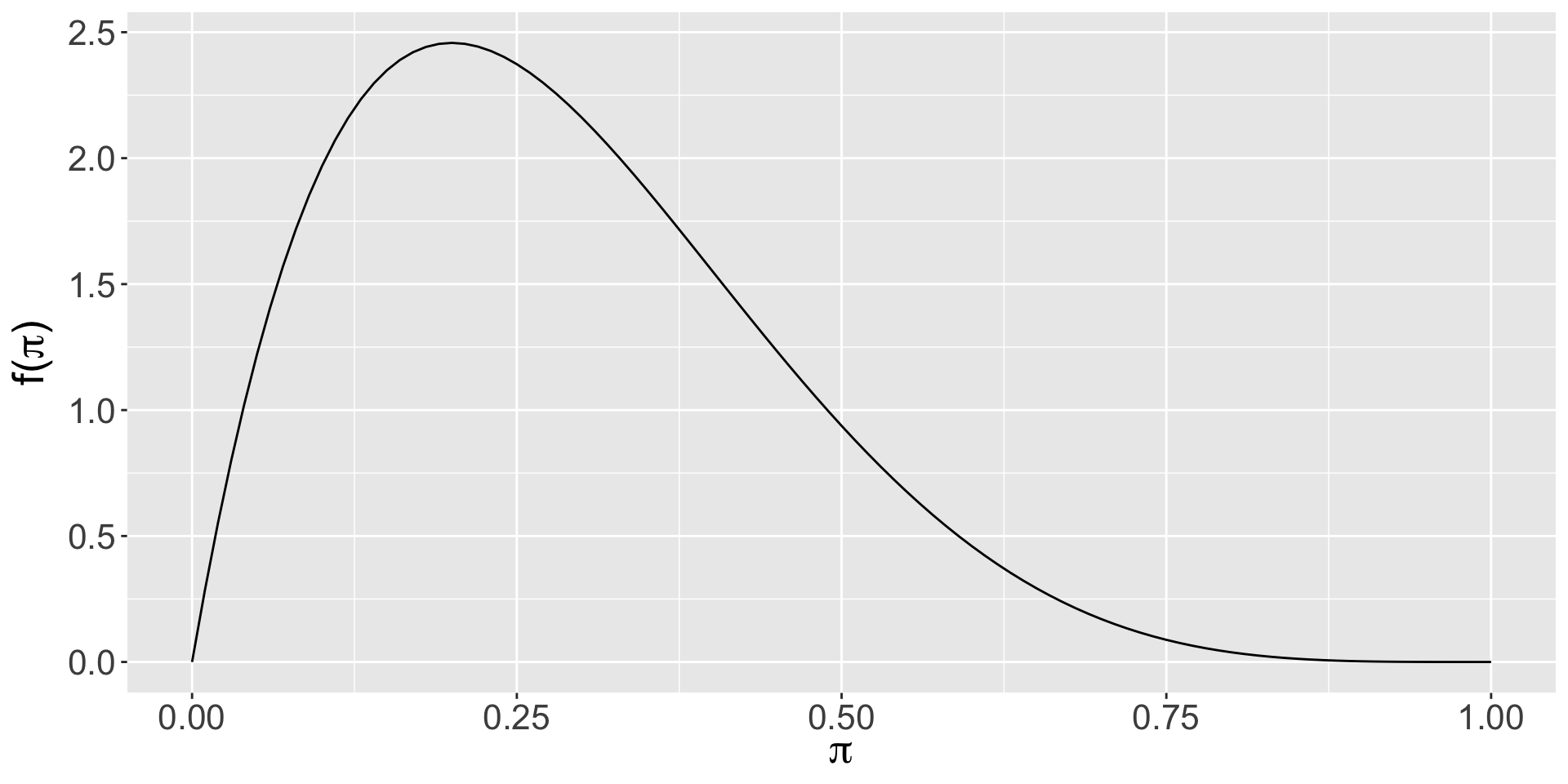
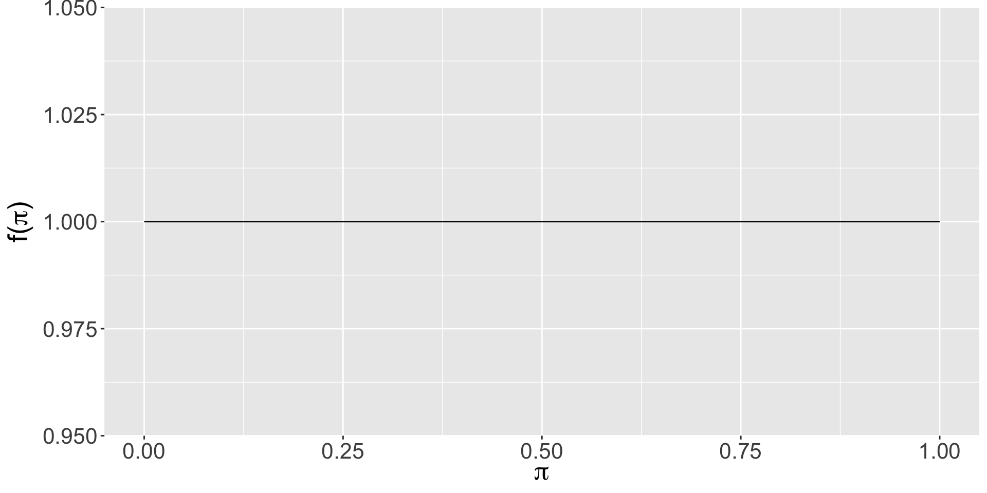
For each of the following students’ prior ideas for \(\pi\), we plot the pdf of a prior.

Katie thinks that it is extremely difficult to get into this program.
Sha’Carri thinks that it is difficult to get into this program.
Caeleb does not have any strong opinions whether it is difficult or easy to get into this program.
Sunisa thinks that it is easy to get into this program.
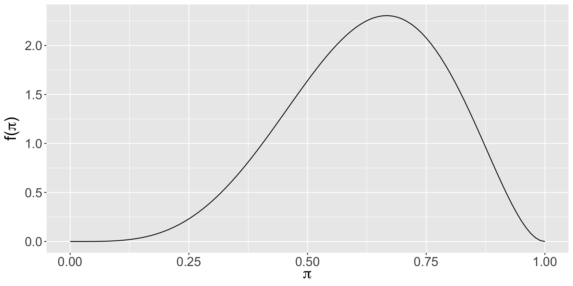
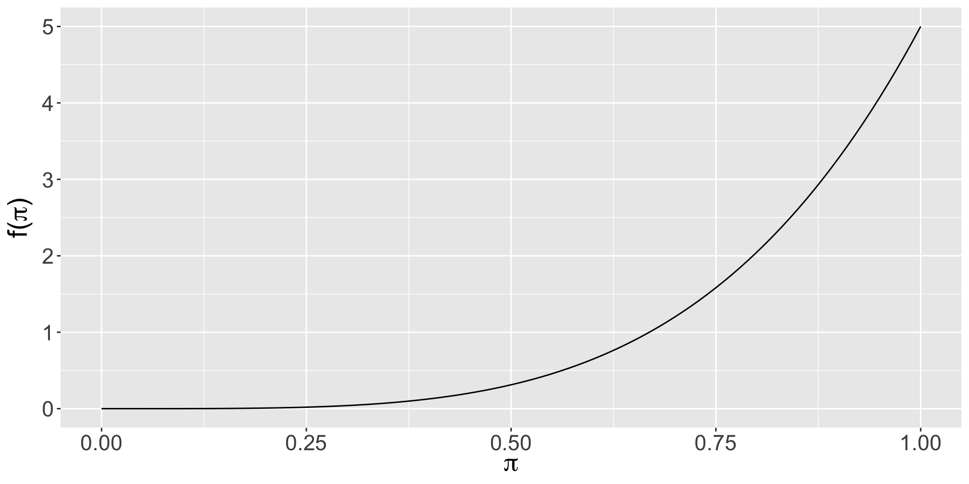
Simone thinks that it is extremely easy to get into this program.

Katie’s prior

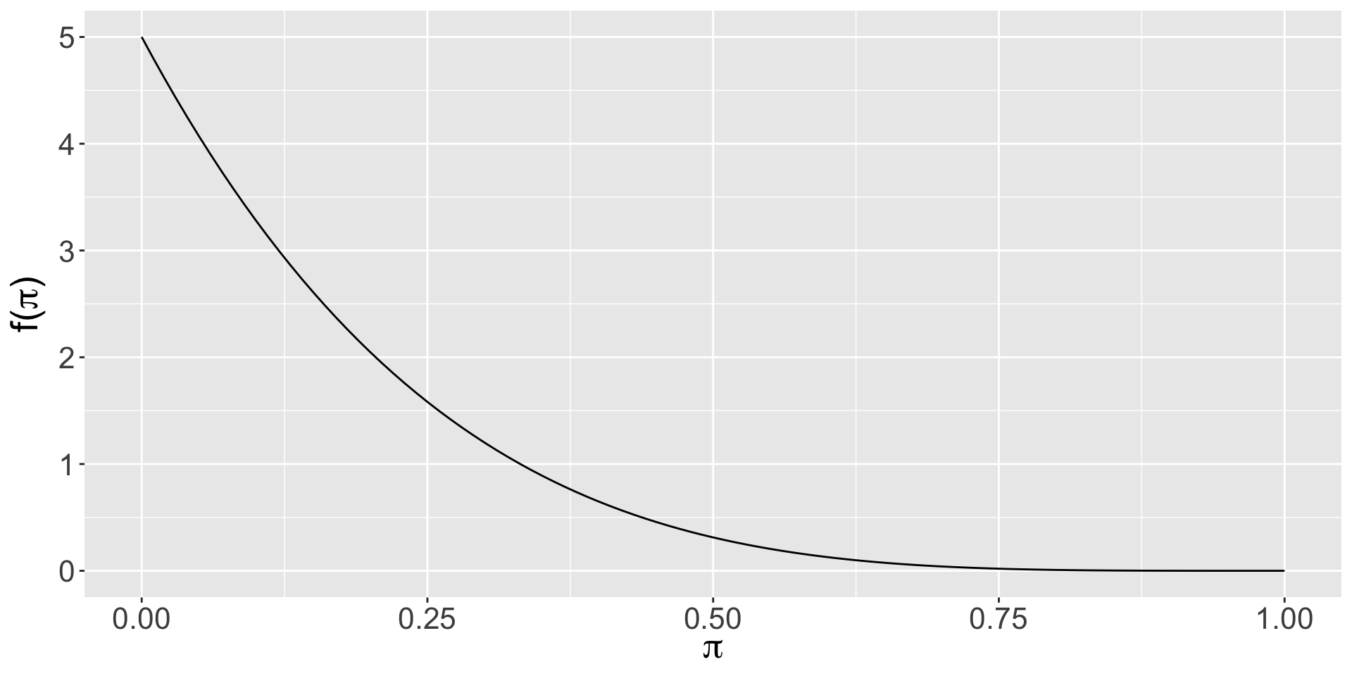
Note: it’s the area under the curve here that represents the probability (the total of which is 1), not the value \(f(\pi)\)

Sha’Carri’s prior

Caeleb’s prior

Sunisa’s prior

Simone’s prior

Beta Prior Model

Let \(\pi\) be a random variable which can take any value between 0 and 1, ie. \(\pi \in [0,1]\). Then the variability in \(\pi\) might be well modeled by a Beta model with shape parameters \(\alpha > 0\) and \(\beta > 0\):

\[\pi \sim \text{Beta}(\alpha, \beta)\] The Beta model is specified by continuous pdf \[\begin{equation} f(\pi) = \frac{\Gamma(\alpha + \beta)}{\Gamma(\alpha)\Gamma(\beta)} \pi^{\alpha-1} (1-\pi)^{\beta-1} \;\; \text{ for } \pi \in [0,1] \end{equation}\] where \(\Gamma(z) = \int_0^\infty y^{z-1}e^{-y}dy\) and \(\Gamma(z + 1) = z \Gamma(z)\). Fun fact: when \(z\) is a positive integer, then \(\Gamma(z)\) simplifies to \(\Gamma(z) = (z-1)!\)

Beta Prior Model

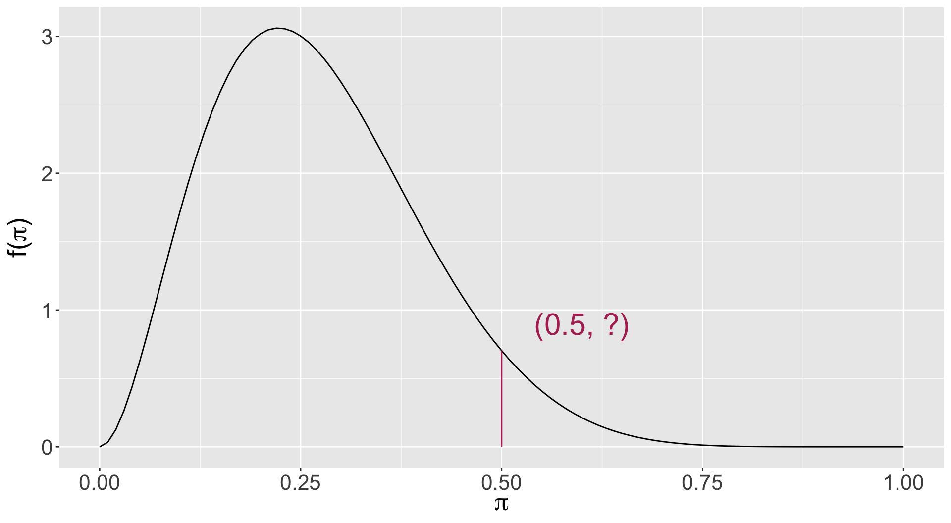
\(\pi \sim \text{Beta}(3, 8)\)

\(f(\pi) = \frac{\Gamma(\alpha + \beta)}{\Gamma(\alpha)\Gamma(\beta)} \pi^{\alpha-1} (1-\pi)^{\beta-1}\)

\(f(\pi) = \frac{\Gamma(3 + 11)}{\Gamma(3)\Gamma(8)} 0.5^{3-1} (1-0.5)^{8-1}\)

\(f(\pi) = \frac{13!}{2!7!} 0.5^{3-1} (1-0.5)^{8-1}\)

\(f(\pi) = 0.703125\)

Beta Prior Model

\(\pi \sim \text{Beta}(3, 8)\)

dbeta(x = 0.5, 
      shape1 = 3, 
      shape2 = 8)

[1] 0.703125

Plotting the Beta Prior

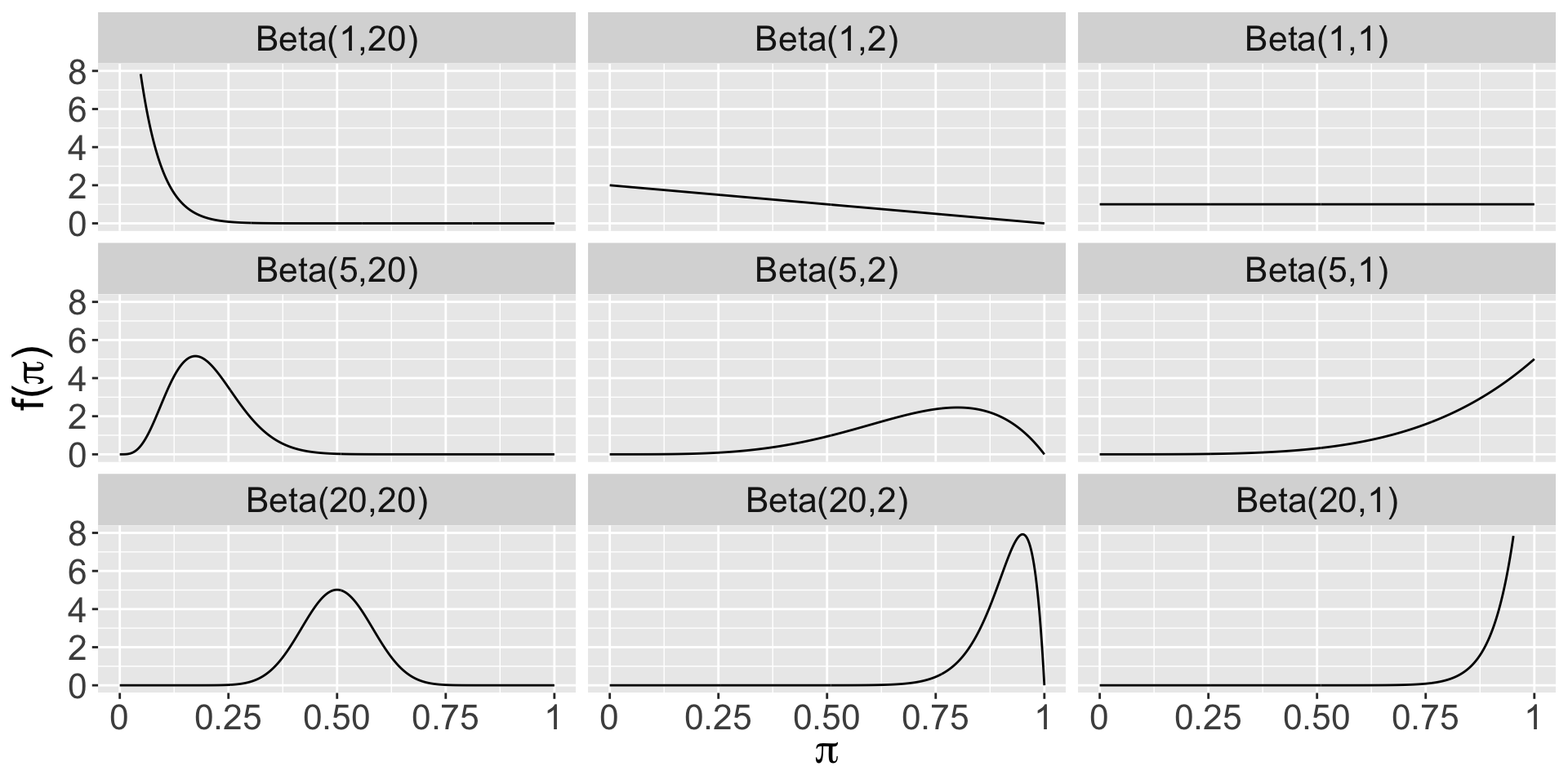
Plotting the Beta Prior with `bayesrules` package

Use the plot_beta() function in the bayesrules package to try different shape parameters. Example:

Code
Plot

plot_beta(alpha = 5, beta = 7)

Beta Descriptives

\[E(\pi) = \frac{\alpha}{\alpha + \beta}\]

\[\text{Mode}(\pi) = \frac{\alpha - 1}{\alpha + \beta - 2}\]

\[\text{Var}(\pi) = \frac{\alpha \beta}{(\alpha + \beta)^2(\alpha + \beta + 1)}\]

Beta Descriptives with `bayesrules` package

Use the summarize_beta() function in the bayesrules package to find the mean, mode, and variance of various Beta distributions. Example:

```{r}
summarize_beta(alpha = 5, beta = 7)
```

       mean mode        var        sd
1 0.4166667  0.4 0.01869658 0.1367354

The Beta-Binomial Model

Graduate Admissions

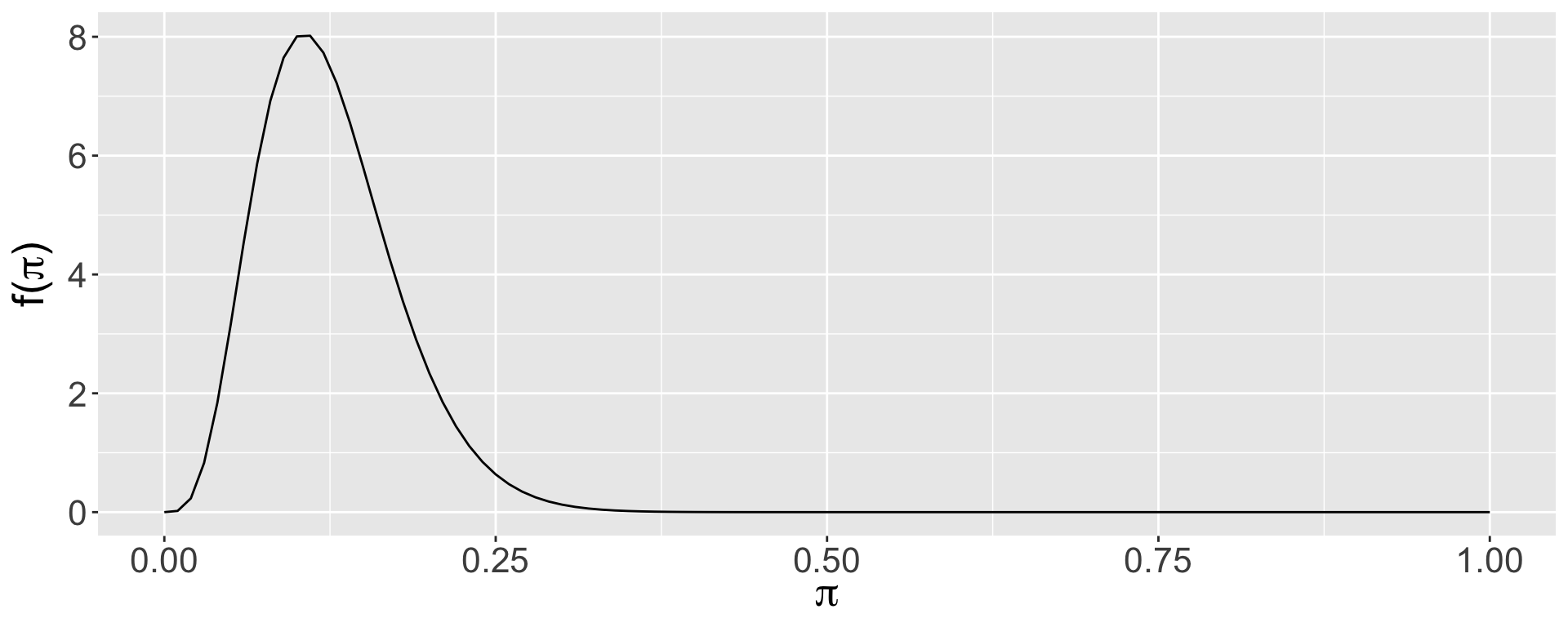
An applicant to a small graduate program wants to know \(\pi\), the probability of admission, so they can determine how many programs to which they should apply. Based on commentary on The GradCafe about similar programs, the applicant thinks that \(\pi\) is likely to be in the range of 0.05 to 0.25.

Plotting the Prior

Discussion question

Is this a reasonable prior choice?

```{r fig.align='center', fig.height=4}
plot_beta(5, 35) +
    theme(text = element_text(size=20)) 
```

Summarizing the Prior

```{r}
summarize_beta(5, 35)
```

   mean      mode         var         sd
1 0.125 0.1052632 0.002667683 0.05164962

Binomial Distribution

The binomial distribution is used to obtain the probability of \(Y=y\) “successes” from a fixed number of \(n\) independent Bernoulli trials.

A Bernoulli trial has two possible outcomes:

one with probability (called the probability of success) \(\pi\), and
the other with probability (called the probability of failure) \(1-\pi\).

The distribution is \(P(Y=y)={n \choose y}\pi^y(1-\pi)^{n-y}\) and has mean \(n\pi\) and variance \(n\pi(1-\pi)\).

Posterior for the Beta-Binomial Model

Let \(\pi \sim \text{Beta}(\alpha, \beta)\) and \(Y|n \sim \text{Bin}(n,\pi)\).

\(f(\pi|y) \propto \frac{\Gamma(\alpha+\beta)}{\Gamma(\alpha)\Gamma(\beta)}\pi^{\alpha-1} (1-\pi)^{\beta-1} {n \choose y}\pi^y(1-\pi)^{n-y}\)

\(f(\pi|y) \propto \pi^{(\alpha+y)-1} (1-\pi)^{(\beta+n-y)-1}\)

\(\pi|y \sim \text{Beta}(\alpha +y, \beta+n-y)\)

\(f(\pi|y) = \frac{\Gamma(\alpha+\beta+n)}{\Gamma(\alpha+y)\Gamma(\beta+n-y)} \pi^{(\alpha+y)-1} (1-\pi)^{(\beta+n-y)-1}\)

Conjugate Prior

We say that \(f(\pi)\) is a conjugate prior for \(L(\pi|y)\) if the posterior, \(f(\pi|y) \propto f(\pi)L(\pi|y)\), is from the same model family as the prior.

Thus, the Beta distribution is a conjugate prior for the Binomial likelihood model because the posterior also follows a Beta distribution.

Note that in the likelihood, \(\pi\) is raised to the power of the number of successes, and \(1-\pi\) is raised to the power of the number of failures. The prior has a similar structure, and \(\alpha\) is often interpreted as the approximate prior number of successes, and \(\beta\) is often interpreted as the approximate prior number of failures, with \(\alpha+\beta\) as the approximate prior sample size.

Graduate Program Admissions

The applicant decides to collect some data on social media and identifies 50 people who applied to the program and asks them whether they were accepted or not. It turns out that 25 of them were! What is the posterior distribution of \(\pi\) after having observed this data?

\(\pi|y \sim \text{Beta}(\alpha +y, \beta+n-y)\)

\(\pi|y \sim \text{Beta}(5 +25, 35+50-25)\)

\(\pi|y \sim \text{Beta}(30, 60)\)

Plotting the Posterior

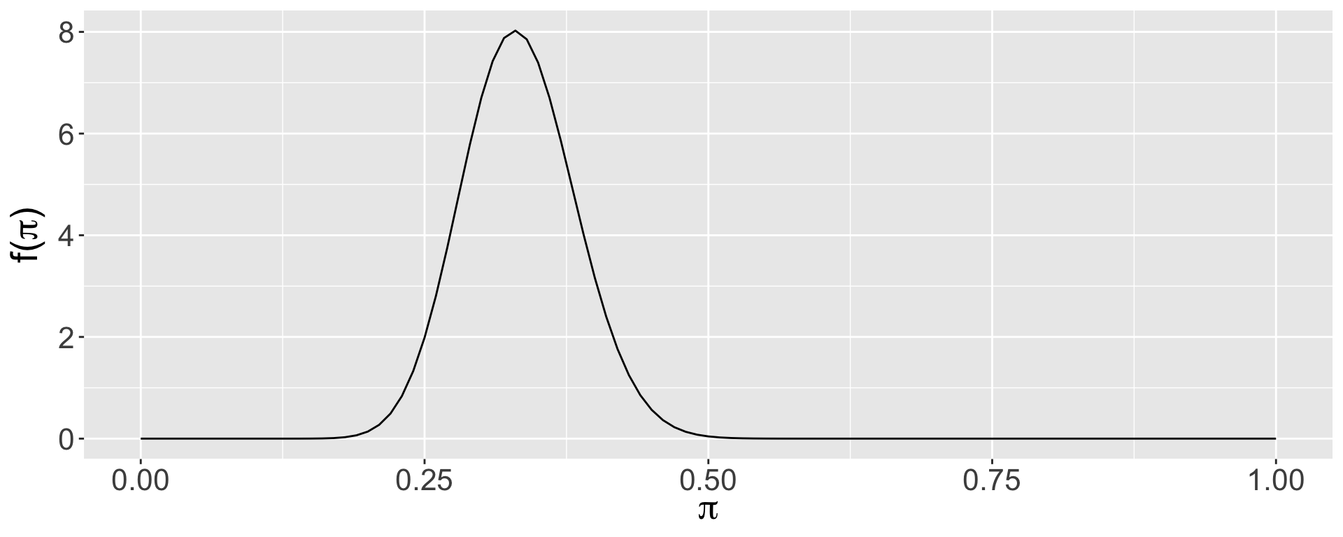
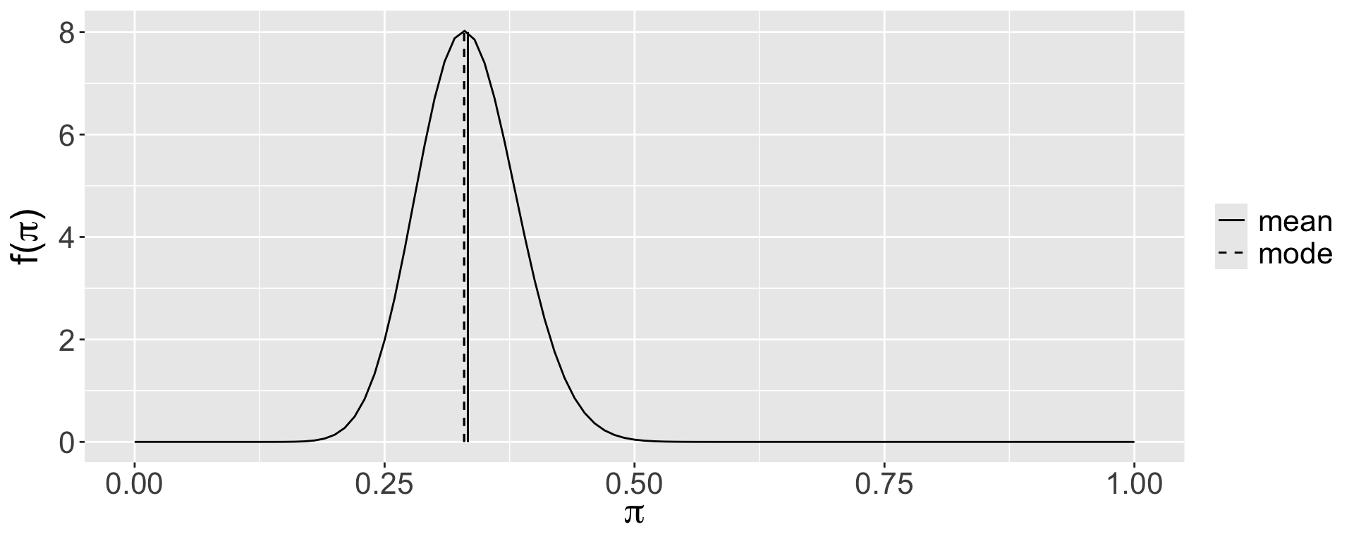
Summarizing the Posterior

       mean      mode         var         sd
1 0.3333333 0.3295455 0.002442002 0.04941662

Plot Summary

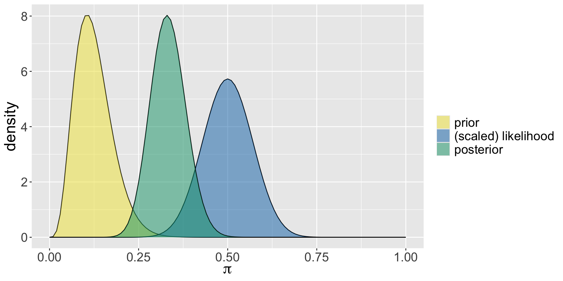
Balancing Act

Posterior Descriptives

\(\pi|(Y=y) \sim \text{Beta}(\alpha+y, \beta+n-y)\)

\[E(\pi | (Y=y)) = \frac{\alpha + y}{\alpha + \beta + n}\] \[\text{Mode}(\pi | (Y=y)) = \frac{\alpha + y - 1}{\alpha + \beta + n - 2} \] \[\text{Var}(\pi | (Y=y)) = \frac{(\alpha + y)(\beta + n - y)}{(\alpha + \beta + n)^2(\alpha + \beta + n + 1)}\\\]

Descriptives of the Posterior

What are the descriptive measures (expected value, mode, and variance) of the posterior distribution for the admissions example?

      model alpha beta      mean      mode         var         sd
1     prior     5   35 0.1250000 0.1052632 0.002667683 0.05164962
2 posterior    30   60 0.3333333 0.3295455 0.002442002 0.04941662

Balance in Bayesian Analysis

Bechdel Test

(Example from bayesrulesbook.com)

Alison Bechdel’s 1985 comic Dykes to Watch Out For has a strip called The Rule, in which a person states that they only go to a movie if it satisfies the following three rules:

the movie has to have at least two women in it;
these two women talk to each other; and
they talk about something besides a man.

This test is now used for assessing movies in terms of representation of women. Even though there are three criteria, a movie either fails (does not satisfy one or more criteria) or passes (satisfies all three criteria) the Bechdel test.

Different Priors, Different Posteriors

Let \(\pi\) be the the proportion of movies that pass the Bechdel test.

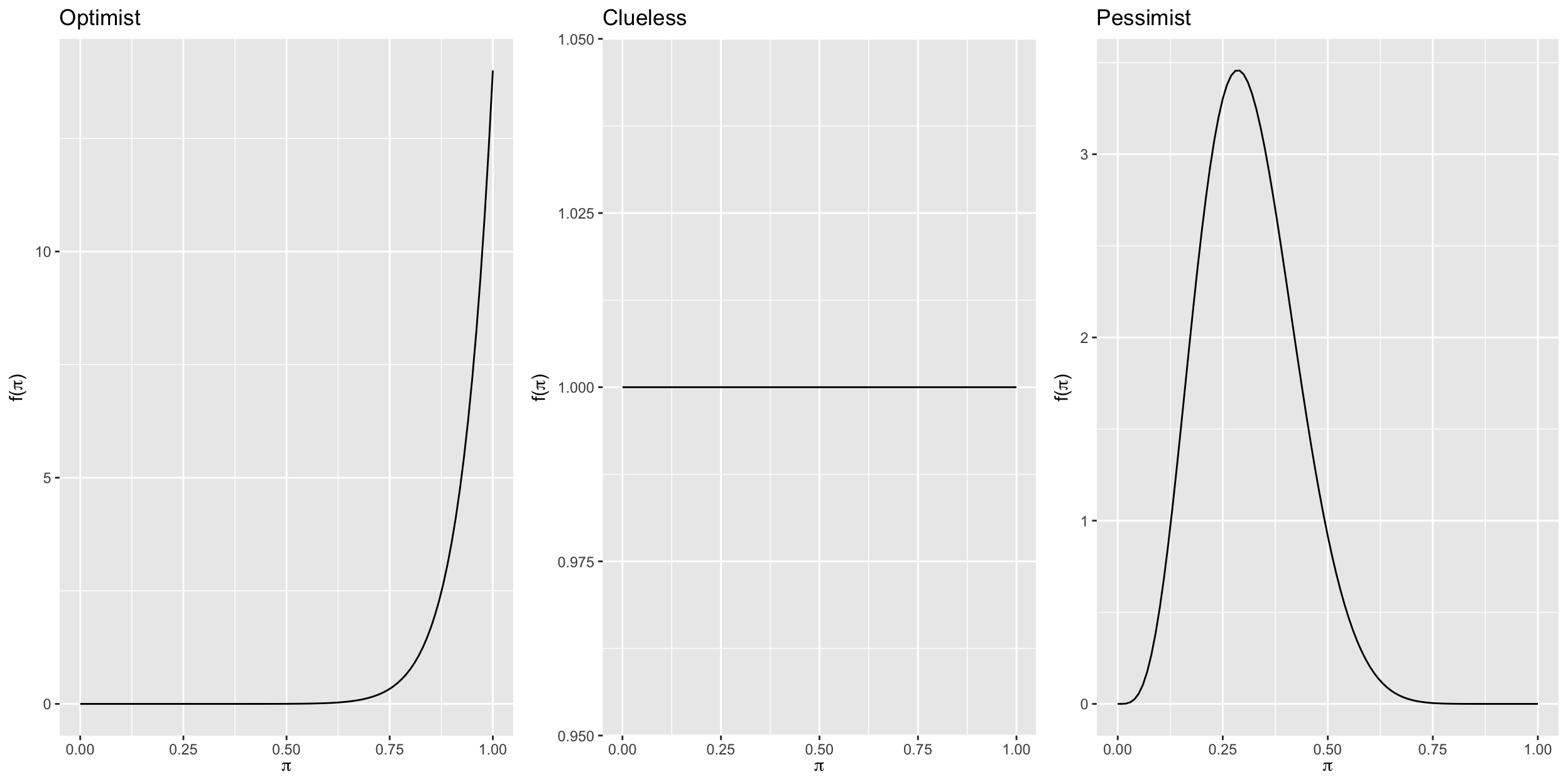
The table shows three different people with three different priors about \(\pi\).

Optimist	Clueless	Pessimist
Beta(14,1)	Beta(1,1)	Beta(5,11)

Next we plot their priors.

Priors

Vocabulary

Informative prior: An informative prior reflects specific information about the unknown variable with high certainty (ie. low variability).

Vague (diffuse) prior: A vague or diffuse prior reflects little specific information about the unknown variable. A flat prior, which assigns equal prior plausibility to all possible values of the variable, is a special case.

Data

library(bayesrules) has the bechdel data frame. Randomly select 20 movies from this dataset (seed = 84735) to be our data
Based on the observed data, we will update the posterior for all three people
We calculate the summary statistics for the prior and the posterior for all three
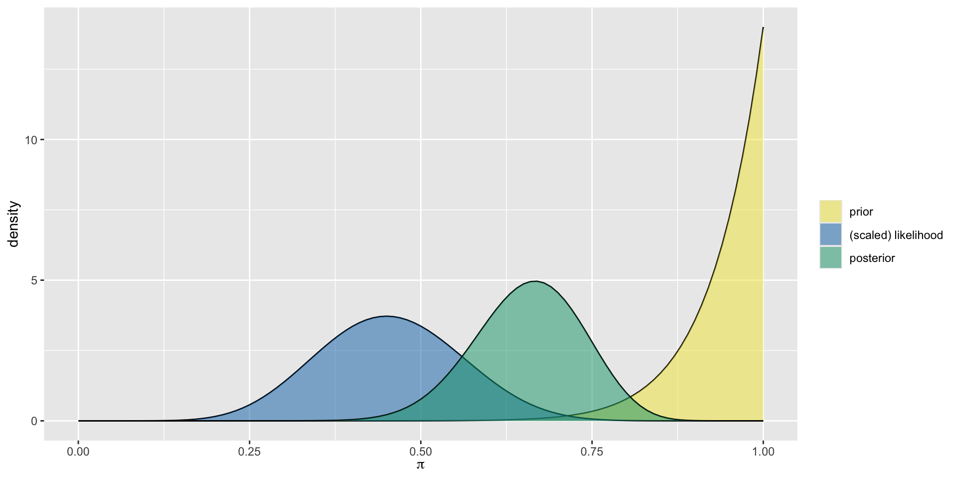
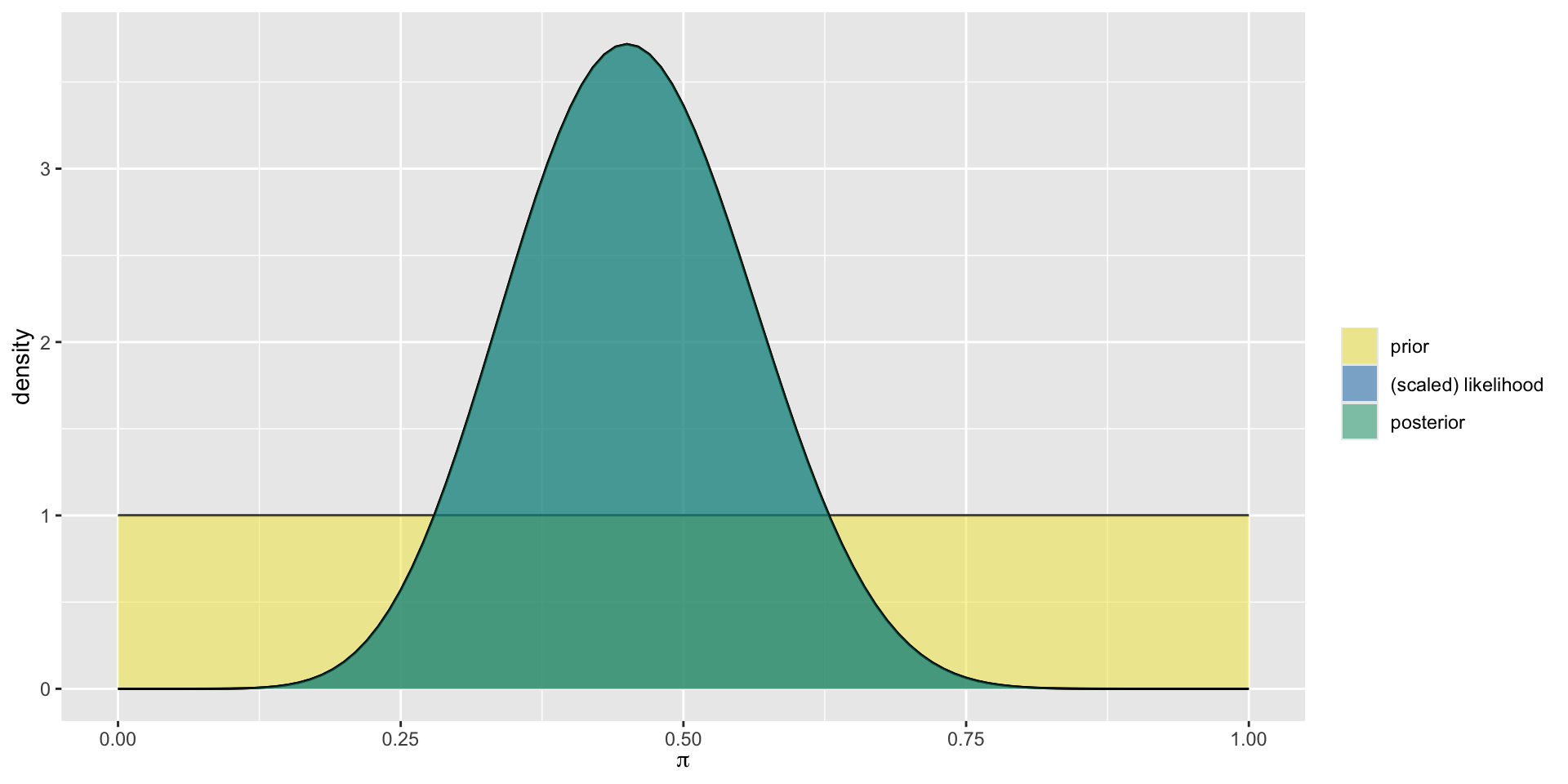
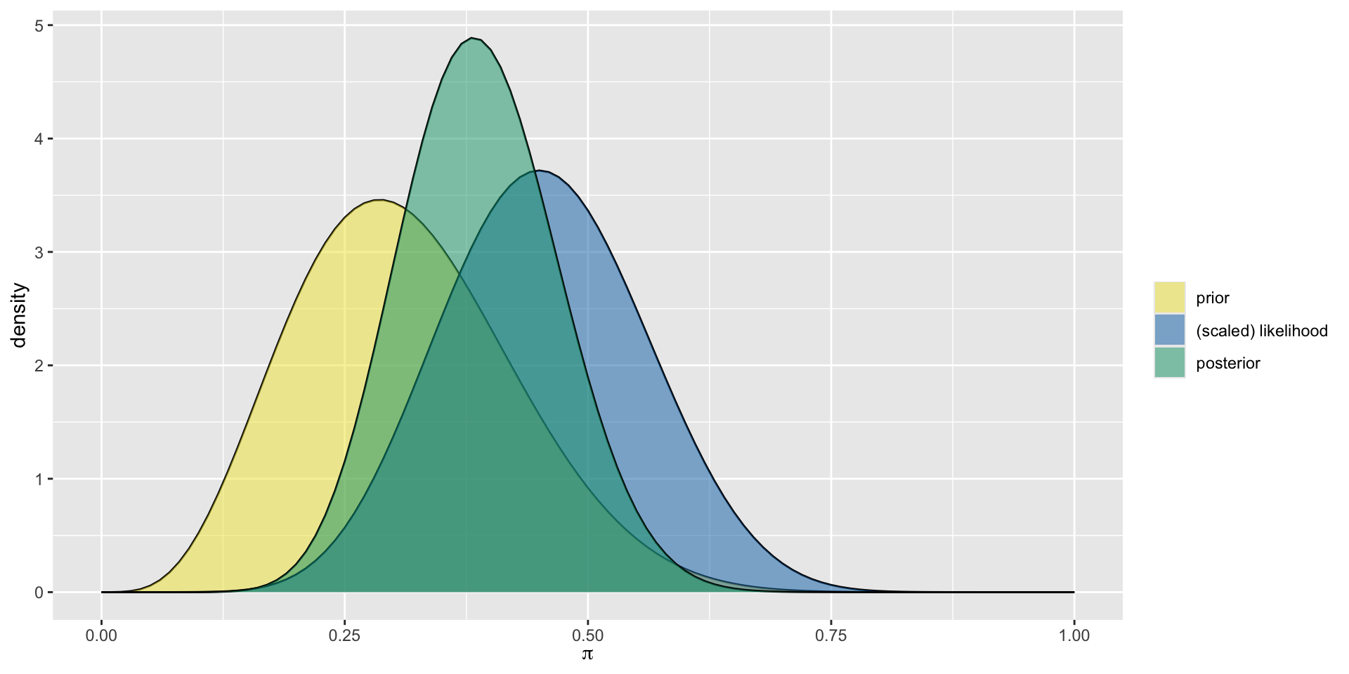
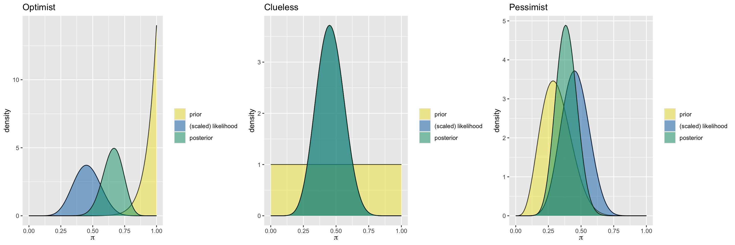
We plot the prior, likelihood, and the posterior for all three
We explain the effect of different priors on the posterior

library(tidyverse)
library(bayesrules)
set.seed(84735)

bechdel_sample <- sample_n(bechdel, 20)

count(bechdel_sample, binary)

# A tibble: 2 × 2
  binary     n
  <chr>  <int>
1 FAIL      11
2 PASS       9

The Optimist

      model alpha beta      mean      mode         var         sd
1     prior    14    1 0.9333333 1.0000000 0.003888889 0.06236096
2 posterior    23   12 0.6571429 0.6666667 0.006258503 0.07911070

The Optimist

The Clueless

      model alpha beta      mean mode        var        sd
1     prior     1    1 0.5000000  NaN 0.08333333 0.2886751
2 posterior    10   12 0.4545455 0.45 0.01077973 0.1038255

The Clueless

The Pessimist

      model alpha beta      mean      mode        var         sd
1     prior     5   11 0.3125000 0.2857143 0.01263787 0.11241827
2 posterior    14   22 0.3888889 0.3823529 0.00642309 0.08014418

The Pessimist

Comparison

Different Data, Different Posteriors

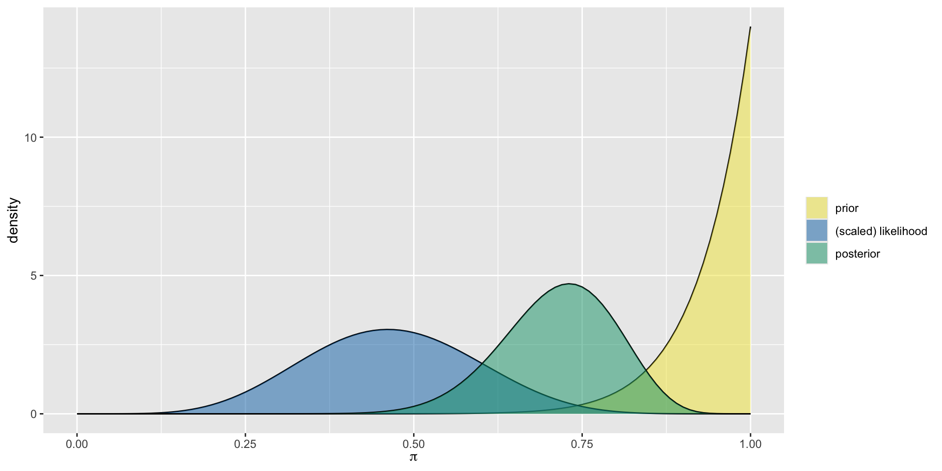
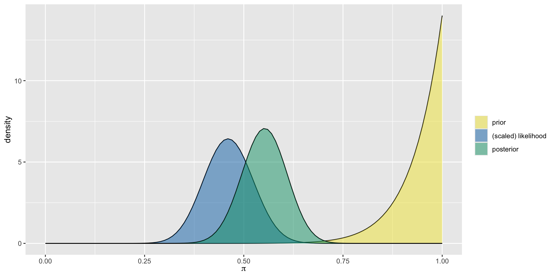
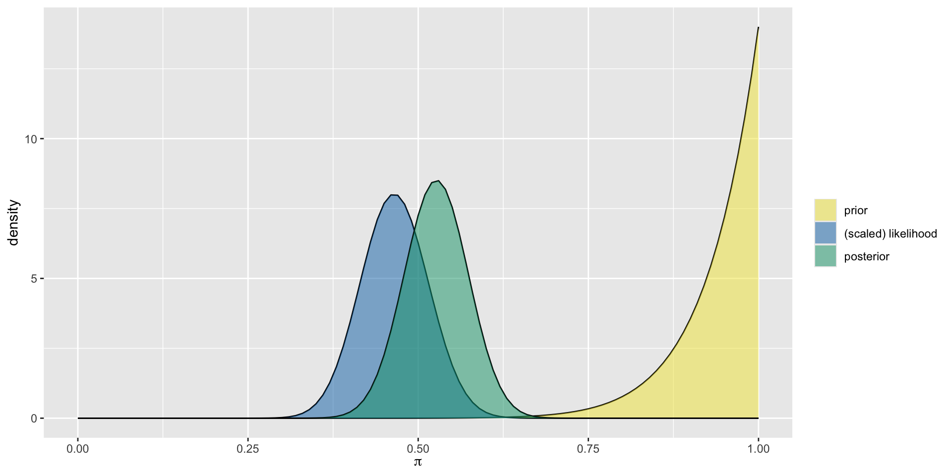
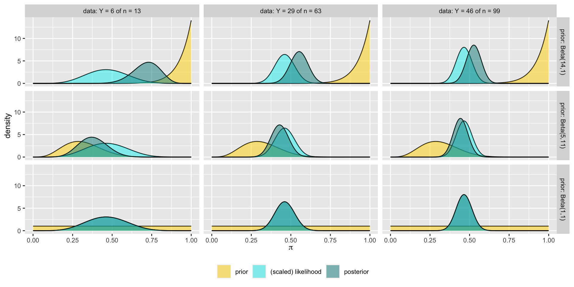
Quincy, Steph, and Noah all share the optimistic Beta(14,1) prior for \(\pi\) but each have access to different data. Quincy reviews movies from 1991. Steph reviews movies from 2000, and Noah reviews movies from 2013. How will the posterior distribution for each differ?

Quincy’s Data

bechdel_1991 <- filter(bechdel, year == 1991)
count(bechdel_1991, binary)

# A tibble: 2 × 2
  binary     n
  <chr>  <int>
1 FAIL       7
2 PASS       6

6/13

[1] 0.4615385

Quincy’s Analysis

Steph’s Data

bechdel_2000 <- filter(bechdel, year == 2000)
count(bechdel_2000, binary)

# A tibble: 2 × 2
  binary     n
  <chr>  <int>
1 FAIL      34
2 PASS      29

29/(34+29)

[1] 0.4603175

Steph’s Analysis

Noah’s Data

bechdel_2013 <- filter(bechdel, year == 2013)
count(bechdel_2013, binary)

# A tibble: 2 × 2
  binary     n
  <chr>  <int>
1 FAIL      53
2 PASS      46

46/(53+46)

[1] 0.4646465

Noah’s Analysis

Summary

Sequential Updating

Sequential Analysis

In a sequential Bayesian analysis, a posterior model is updated incrementally as more data comes in. With the introduction of each new piece of data, the previous posterior model reflecting our understanding prior to observing this data becomes the new prior model.

Time Travel to the End of 1970

Suppose our prior a movie passes the Bechdel test is an optimistic \(\pi \sim Beta(14,1)\). Now let’s look at the 1970 movies.

bechdel %>% 
  filter(year == 1970)

# A tibble: 1 × 3
   year title                          binary
  <dbl> <chr>                          <chr> 
1  1970 Beyond the Valley of the Dolls PASS

The Posterior

summarize_beta_binomial(14, 1, y = 1, n = 1)

      model alpha beta      mean mode         var         sd
1     prior    14    1 0.9333333    1 0.003888889 0.06236096
2 posterior    15    1 0.9375000    1 0.003446691 0.05870853

At the End of 1971

Our posterior at the end of 1970 becomes our new 1971 prior, incorporating the 1970 data, given by \(\pi \sim Beta(15,1)\)

Let’s look at the 1971 movies that have been rated.

bechdel %>% 
  filter(year == 1971)

# A tibble: 5 × 3
   year title                                   binary
  <dbl> <chr>                                   <chr> 
1  1971 Escape from the Planet of the Apes      FAIL  
2  1971 Shaft                                   FAIL  
3  1971 Straw Dogs                              FAIL  
4  1971 The French Connection                   FAIL  
5  1971 Willy Wonka &amp; the Chocolate Factory FAIL

The Posterior

summarize_beta_binomial(15, 1, y = 0, n = 5)

      model alpha beta      mean      mode         var         sd
1     prior    15    1 0.9375000 1.0000000 0.003446691 0.05870853
2 posterior    15    6 0.7142857 0.7368421 0.009276438 0.09631427

At the End of 1972

New prior incorporating 1971 data: \(\pi \sim Beta(15,6)\)

bechdel %>% 
  filter(year == 1972)

# A tibble: 3 × 3
   year title          binary
  <dbl> <chr>          <chr> 
1  1972 1776           FAIL  
2  1972 Pink Flamingos PASS  
3  1972 The Godfather  FAIL

The Posterior

summarize_beta_binomial(15, 6, y = 1, n = 3)

      model alpha beta      mean      mode         var         sd
1     prior    15    6 0.7142857 0.7368421 0.009276438 0.09631427
2 posterior    16    8 0.6666667 0.6818182 0.008888889 0.09428090

Summary

Time	Data	Model
before the analysis	NA	Beta(14,1)
at the end of 1970	Y = 1, n = 1	Beta(15,1)
at the end of 1971	Y = 0, n = 5	Beta(15, 6)
at the end of 1972	Y = 1, n = 3	Beta(16,8)

Data Order Invariance

Time	Data	Model
before the analysis	NA	Beta(14,1)
1972	Y = 1, n = 3	Beta(15,3)
1971	Y = 0, n = 5	Beta(15,8)
1970	Y = 1, n = 1	Beta(16,8)

As long as we include the same 3 years, our final conclusion is the same!

What If We Observe All the Data at Once?

Time	Data	Model
before the analysis	NA	Beta(14,1)
1970	Y = 1, n = 1
1971	Y = 0, n = 5
1972	Y = 1, n = 3
Total	Y = 2, n = 9

      model alpha beta      mean      mode         var         sd
1     prior    14    1 0.9333333 1.0000000 0.003888889 0.06236096
2 posterior    16    8 0.6666667 0.6818182 0.008888889 0.09428090

Sequential Updating

Let \(\theta\) be any parameter of interest with prior pdf \(f(\theta)\). Then a sequential analysis in which we first observe a data point \(y_1\) and then a second data point \(y_2\) will produce the same posterior model of \(\theta\) as if we first observed \(y_2\) and then \(y_1\):

\[f(\theta | y_1,y_2) = f(\theta|y_2,y_1)\;.\]

Similarly, the posterior model is invariant to whether we observe the data all at once or sequentially.

Discrete Response Data

The Beta Prior Distribution

Back to Graduate School Applications

Continuous Probability Models

Plotting the Continuous Prior

Katie’s prior

Sha’Carri’s prior

Caeleb’s prior

Sunisa’s prior

Simone’s prior

Beta Prior Model

Beta Prior Model

Beta Prior Model

Plotting the Beta Prior

Plotting the Beta Prior with bayesrules package

Beta Descriptives

Beta Descriptives with bayesrules package

The Beta-Binomial Model

Graduate Admissions

Plotting the Prior

Summarizing the Prior

Binomial Distribution

Posterior for the Beta-Binomial Model

Conjugate Prior

Graduate Program Admissions

Plotting the Posterior

Summarizing the Posterior

Plot Summary

Balancing Act

Posterior Descriptives

Descriptives of the Posterior

Balance in Bayesian Analysis

Bechdel Test

Different Priors, Different Posteriors

Priors

Vocabulary

Data

The Optimist

The Optimist

The Clueless

The Clueless

The Pessimist

The Pessimist

Comparison

Different Data, Different Posteriors

Quincy’s Data

Quincy’s Analysis

Steph’s Data

Steph’s Analysis

Noah’s Data

Noah’s Analysis

Summary

Sequential Updating

Sequential Analysis

Time Travel to the End of 1970

The Posterior

At the End of 1971

The Posterior

At the End of 1972

The Posterior

Summary

Data Order Invariance

What If We Observe All the Data at Once?

Sequential Updating

Plotting the Beta Prior with `bayesrules` package

Beta Descriptives with `bayesrules` package