Evaluating
regression models
Day 4
Note that examples in this part of the lecture are a simplified version of Chapter 10 of Bayes Rules! book.
Packages
How fair is the model? How was the data collected? By whom and for what purpose? How might the results of the analysis, or the data collection itself, impact individuals and society? What biases or power structures might be baked into this analysis?
How wrong is the model? George Box famously said: “All models are wrong, but some are useful.” What’s important to know then is, how wrong is our model? Are our model assumptions reasonable?
How accurate are the posterior predictive models?
Checking Model Assumptions
\[Y_i | \beta_0, \beta_1, \sigma \stackrel{ind}{\sim} N(\mu_i, \sigma^2) \;\; \text{ with } \;\; \mu_i = \beta_0 + \beta_1 X_i .\]
- Conditioned on \(X\), the observed data \(Y_i\) on case \(i\) is independent of the observed data on any other case \(j\).
- The typical \(Y\) outcome can be written as a linear function of \(X\), \(\mu = \beta_0 + \beta_1 X\).
- At any \(X\) value, \(Y\) varies normally around \(\mu\) with consistent variability \(\sigma\).
Independence
When taken alone, ridership \(Y\) is likely correlated over time – today’s ridership likely tells us something about tomorrow’s ridership. Yet much of this correlation, or dependence, can be explained by the time of year and features associated with the time of year – like temperature \(X\). Thus, knowing the temperature on two subsequent days may very well “cancel out” the time correlation in their ridership data.
Linearity and Constant Variance

The relationship between ridership and temperature does appear to be linear. Further, with the slight exception of colder days on which ridership is uniformly small, the variability in ridership does appear to be roughly consistent across the range of temperatures \(X\).
Posterior predictive check
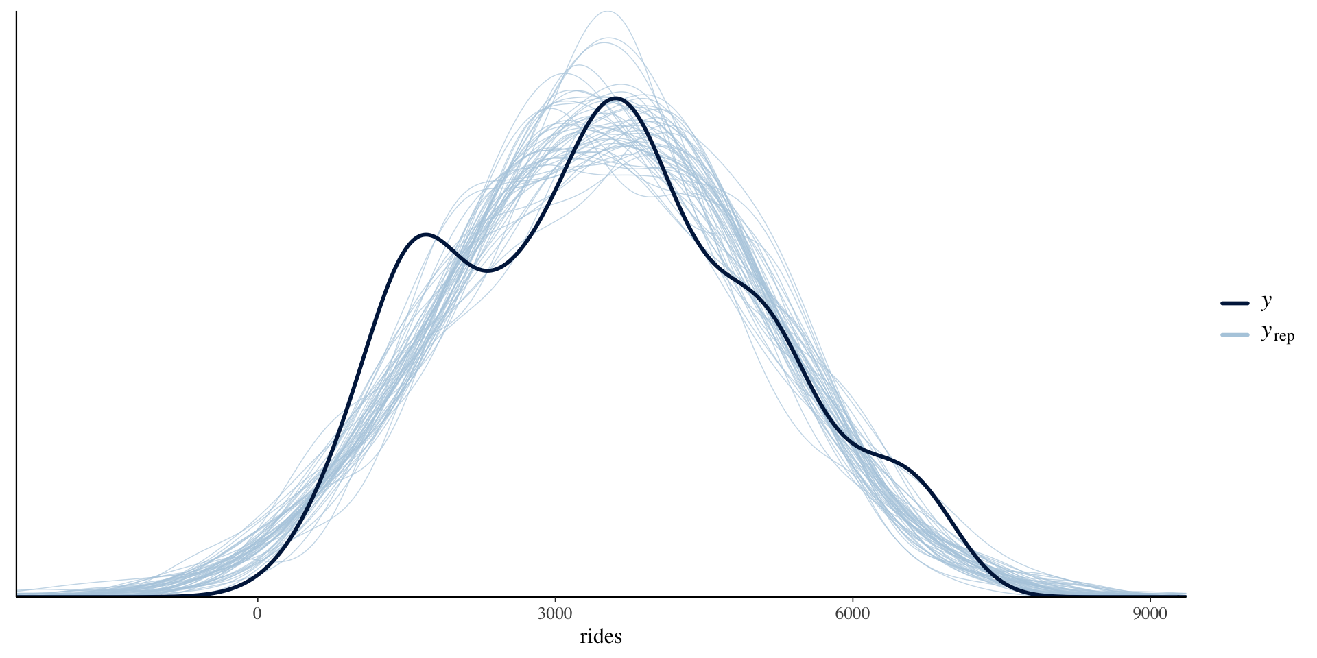
Consider a regression model with response variable \(Y\), predictor \(X\), and a set of regression parameters \(\theta\). For example, in the model in the previous slides \(\theta = (\beta_0,\beta_1,\sigma)\). Further, let \(\left\lbrace \theta^{(1)}, \theta^{(2)}, \ldots, \theta^{(N)}\right\rbrace\) be an \(N\)-length Markov chain for the posterior model of \(\theta\). Then a “good” Bayesian model will produce predictions of \(Y\) with features similar to the original \(Y\) data. To evaluate whether your model satisfies this goal:
- At each set of posterior plausible parameters \(\theta^{(i)}\), simulate a sample of \(Y\) values from the likelihood model, one corresponding to each \(X\) in the original sample of size \(n\). This produces \(N\) separate samples of size \(n\).
- Compare the features of the \(N\) simulated \(Y\) samples, or a subset of these samples, to those of the original \(Y\) data.
first_set <- head(bike_model_df, 1)
beta_0 <- first_set$`(Intercept)`
beta_1 <- first_set$temp_feel
sigma  <- first_set$sigma
set.seed(84735)
one_simulation <- bikes %>%
  mutate(mu = beta_0 + beta_1 * temp_feel,
         simulated_rides = rnorm(500, mean = mu, sd = sigma)) %>%
  select(temp_feel, rides, simulated_rides)

head(one_simulation, 2)
temp_feel rides simulated_rides
1 64.72625 654 3962.406
2 49.04645 1229 1657.900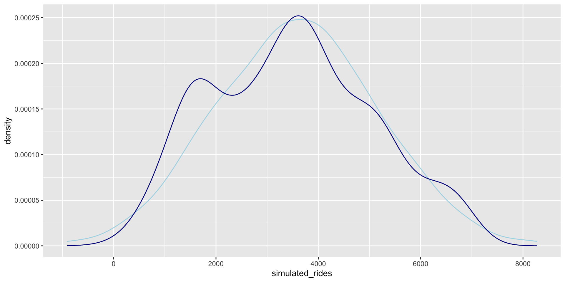
One posterior simulated dataset of ridership (light blue) along with the actual observed ridership data (dark blue)
How accurate are the posterior predictive models?
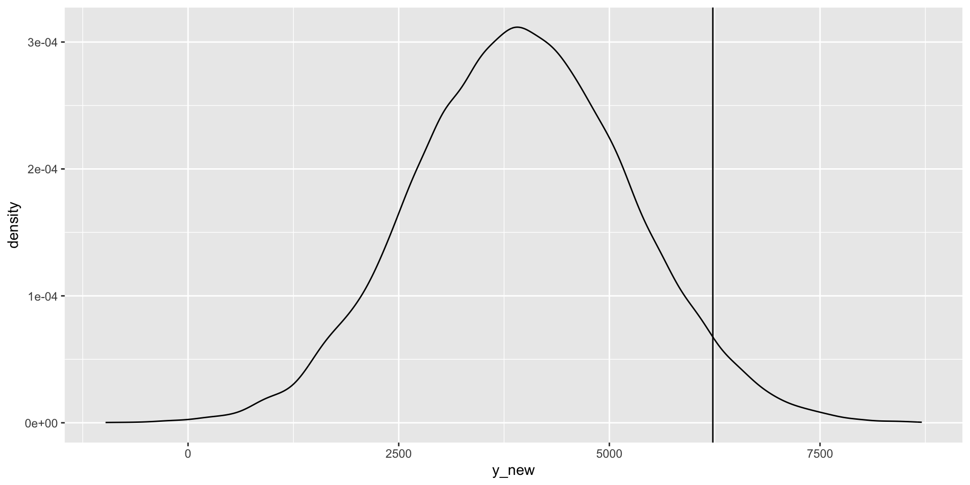
observed value: \(Y\)
posterior predictive mean: \(Y'\)
predictive error: \(Y - Y'\)
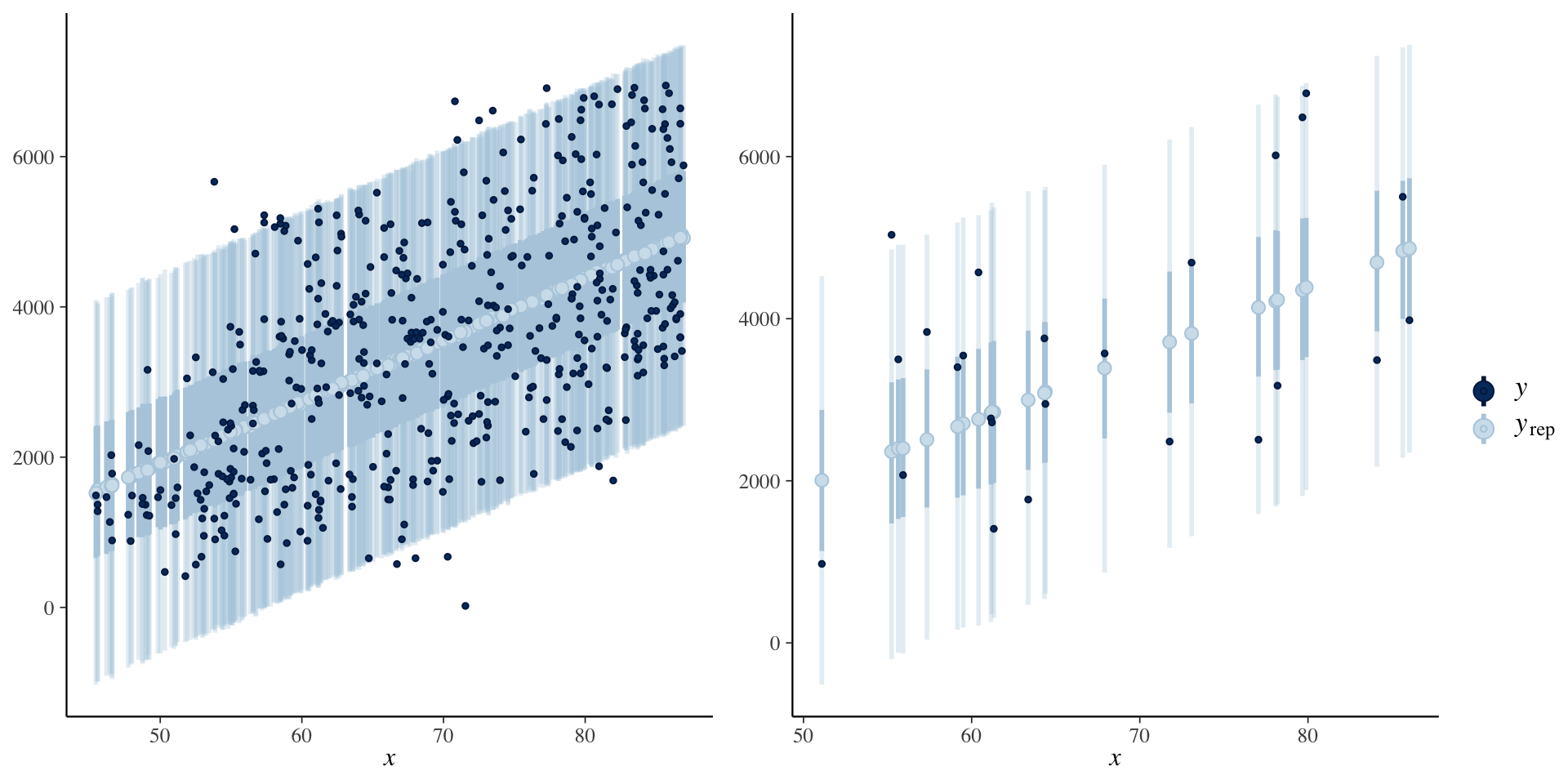
Let \(Y_1, Y_2, \ldots, Y_n\) denote \(n\) observed outcomes. Then each \(Y_i\) has a corresponding posterior predictive model with mean \(Y_i'\) and standard deviation \(\text{sd}_i\). We can evaluate the overall posterior predictive model quality by the following measures:
mae
The median absolute error (MAE) measures the typical difference between the observed \(Y_i\) and their posterior predictive means \(Y_i'\),\[\text{MAE} = \text{median}|Y_i - Y_i'|.\]
mae_scaled
The scaled median absolute error measures the typical number of standard deviations that the observed \(Y_i\) fall from their posterior predictive means \(Y_i'\):\[\text{MAE scaled} = \text{median}\frac{|Y_i - Y_i'|}{\text{sd}_i}.\]
within_50andwithin_95
Thewithin_50statistic measures the proportion of observed values \(Y_i\) that fall within their 50% posterior prediction interval. Thewithin_95statistic is similar, but for 95% posterior prediction intervals.
The k-fold cross validation algorithm
Create folds. Let \(k\) be some integer from 2 to our original sample size \(n\). Split the data into \(k\) folds, or subsets, of roughly equal size.
Train and test the model.
- Train the model using the first \(k - 1\) data folds combined.
- Test this model on the \(k\)th data fold.
- Measure the prediction quality (eg: by MAE).
Repeat. Repeat step 2 \(k - 1\) times, each time leaving out a different fold for testing.
Calculate cross-validation estimates. Steps 2 and 3 produce \(k\) different training models and \(k\) corresponding measures of prediction quality. Average these \(k\) measures to obtain a single cross-validation estimate of prediction quality.
   fold       mae mae_scaled within_50 within_95
1     1  990.0073  0.7707234      0.46      0.98
2     2  965.0892  0.7440878      0.42      1.00
3     3  949.8799  0.7293869      0.42      0.98
4     4 1018.5578  0.7908781      0.46      0.98
5     5 1162.1412  0.9095612      0.36      0.96
6     6  937.1655  0.7323089      0.46      0.94
7     7 1269.2759  1.0047126      0.32      0.96
8     8 1111.8039  0.8603143      0.36      1.00
9     9 1099.9589  0.8679345      0.40      0.92
10 10 786.5296 0.6054229 0.56 0.96Note that examples in this part of the lecture are a simplified version of Chapter 11 of Bayes Rules! book.
Data
Rows: 200
Columns: 6
$ location     <fct> Uluru, Uluru, Uluru, Uluru, Uluru, Uluru, Uluru, Uluru, U…
$ windspeed9am <dbl> 20, 9, 7, 28, 24, 22, 22, 4, 2, 9, 20, 20, 9, 22, 9, 24, …
$ humidity9am  <int> 23, 71, 15, 29, 10, 32, 43, 57, 64, 40, 28, 30, 95, 47, 7…
$ pressure9am  <dbl> 1023.3, 1012.9, 1012.3, 1016.0, 1010.5, 1012.2, 1025.7, 1…
$ temp9am      <dbl> 20.9, 23.4, 24.1, 26.4, 36.7, 25.1, 14.9, 15.9, 24.6, 15.…
$ temp3pm      <dbl> 29.7, 33.9, 39.7, 34.2, 43.3, 33.5, 24.0, 22.6, 33.2, 24.…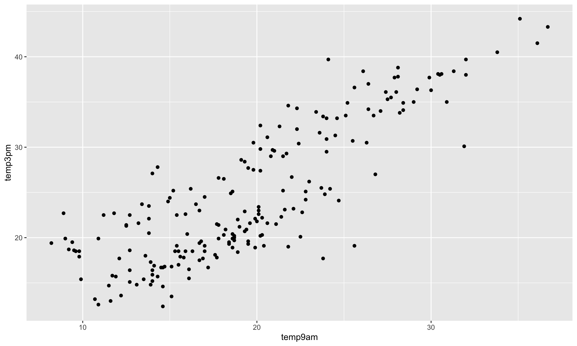
\(\text{likelihood model:} \; \; \; Y_i | \beta_0, \beta_1, \sigma \;\;\;\stackrel{ind}{\sim} N\left(\mu_i, \sigma^2\right)\text{ with } \mu_i = \beta_0 + \beta_1X_{i1}\)
\(\text{prior models:}\)
\(\beta_0\sim N(\ldots, \ldots )\)
\(\beta_1\sim N(\ldots, \ldots )\)
\(\sigma \sim \text{Exp}(\ldots)\)
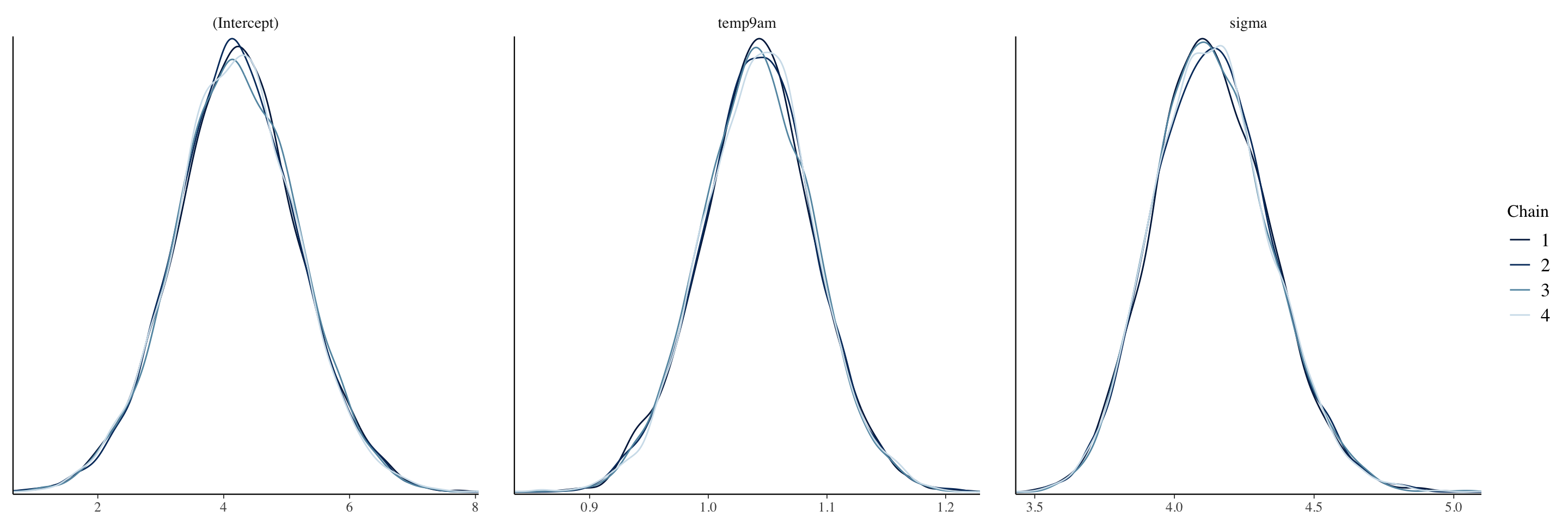
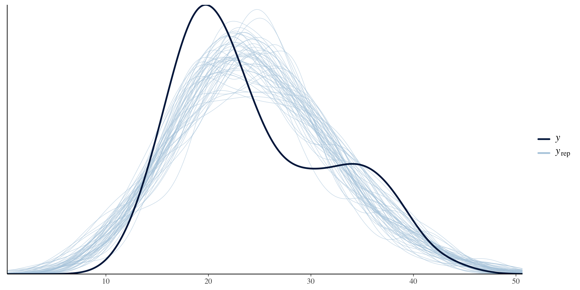
Considering a categorical predictor

\[X_{i2} = \begin{cases} 1 & \text{ Wollongong} \\ 0 & \text{ otherwise (ie. Uluru)} \\ \end{cases}\]
\(\text{likelihood model:} \; \; \; Y_i | \beta_0, \beta_1, \sigma \;\;\;\stackrel{ind}{\sim} N\left(\mu_i, \sigma^2\right)\text{ with } \mu_i = \beta_0 + \beta_1X_{i2}\)
\(\text{prior models:}\)
\(\beta_0\sim N(\ldots, \ldots )\)
\(\beta_1\sim N(\ldots, \ldots )\)
\(\sigma \sim \text{Exp}(\ldots)\)
–
For Uluru, \(X_{i2} = 0\) and the trend in 3pm temperature simplifies to
\[\beta_0 + \beta_1 \cdot 0 = \beta_0 \; .\] For Wollongong, \(X_{i2} = 1\) and the trend in 3pm temperature is
\[\beta_0 + \beta_1 \cdot 1 = \beta_0 + \beta_1 \; .\]
Simulating the Posterior
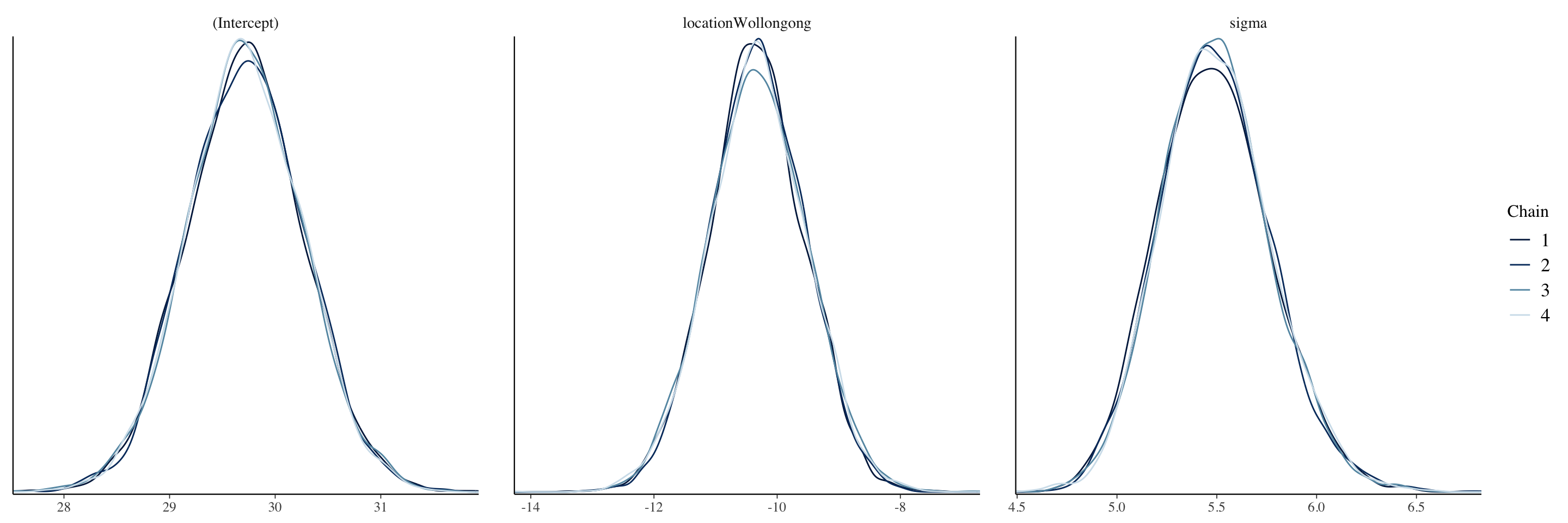
# Posterior summary statistics
model_summary <- summary(weather_model_2)
head(as.data.frame(model_summary), -2) %>%
  select(mean, "10%", "90%", Rhat)
mean 10% 90% Rhat
(Intercept) 29.718920 29.01943 30.424971 1.0000536
locationWollongong -10.317874 -11.31883 -9.301761 1.0001838
sigma 5.494874 5.14486 5.857824 0.9999858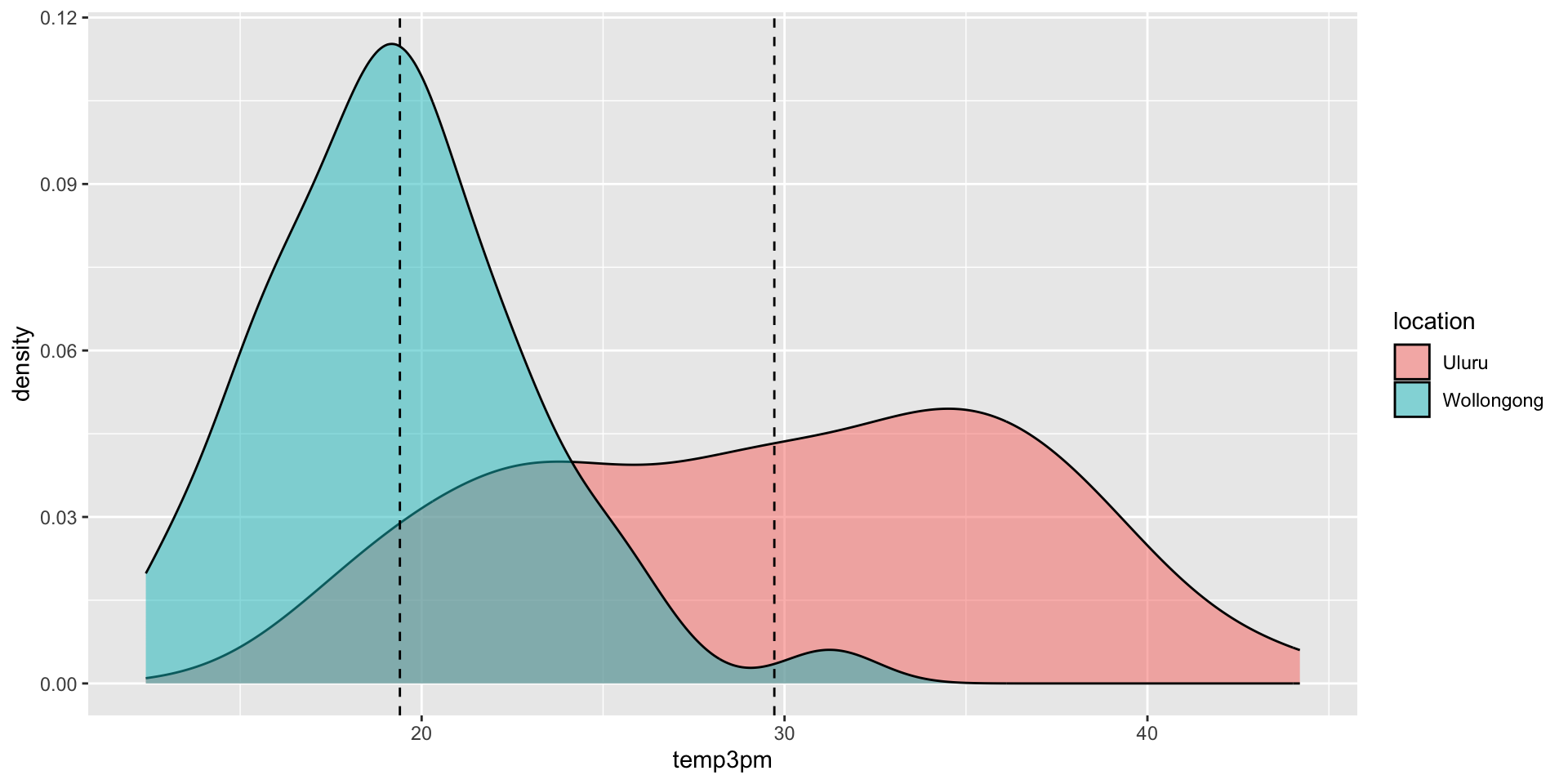
Two Predictors
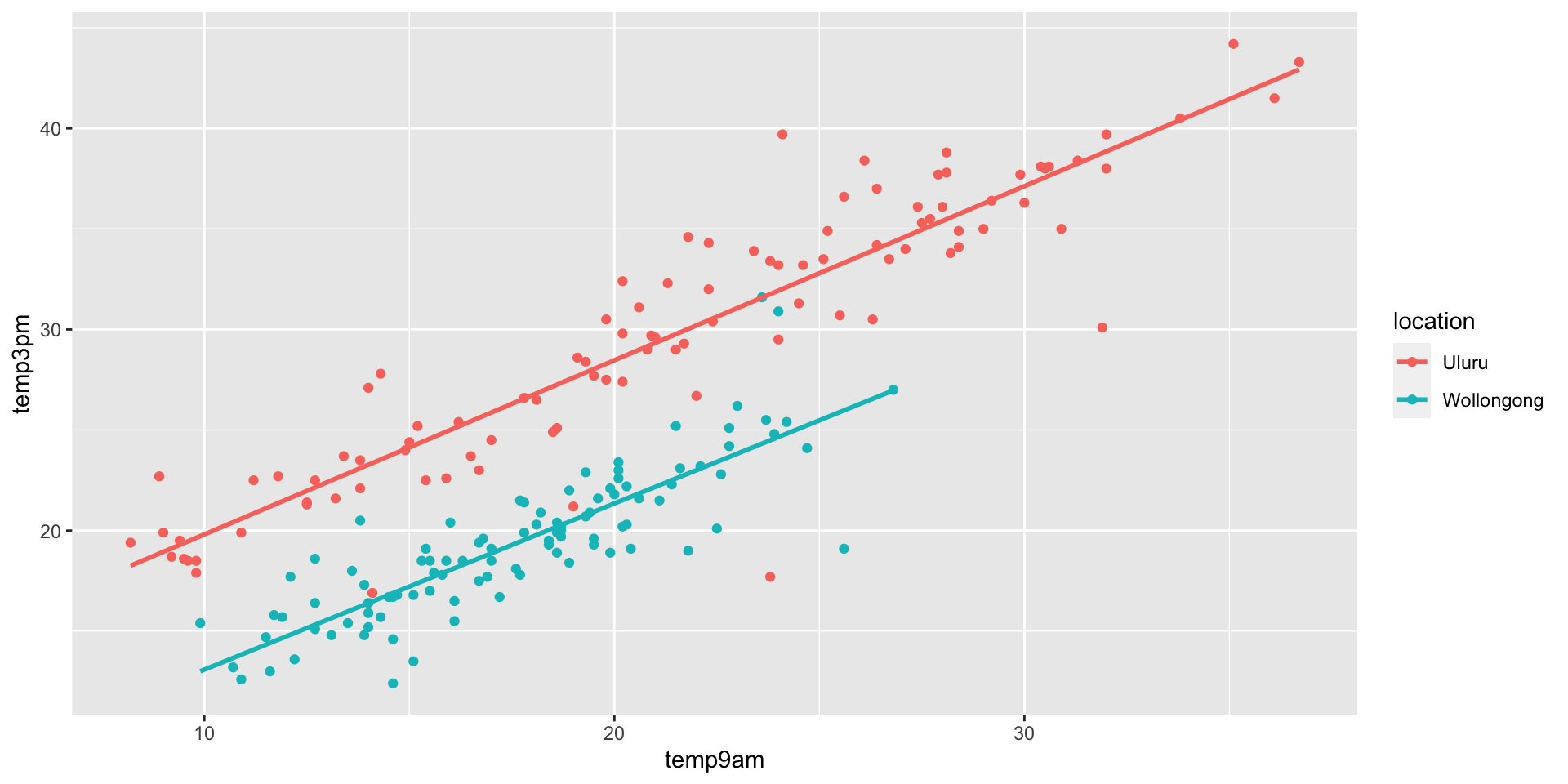
\(\text{likelihood model:}\) \(Y_i | \beta_0, \beta_1, \beta_2 \sigma \;\;\;\stackrel{ind}{\sim} N\left(\mu_i, \sigma^2\right)\text{ with } \mu_i = \beta_0 + \beta_1X_{i1} + \beta_2X_{i2}\)
\(\text{prior models:}\)
\(\beta_0\sim N(m_0, s_0 )\)
\(\beta_1\sim N(m_1, s_1 )\)
\(\beta_2\sim N(m_2, s_2 )\)
\(\sigma \sim \text{Exp}(l)\)
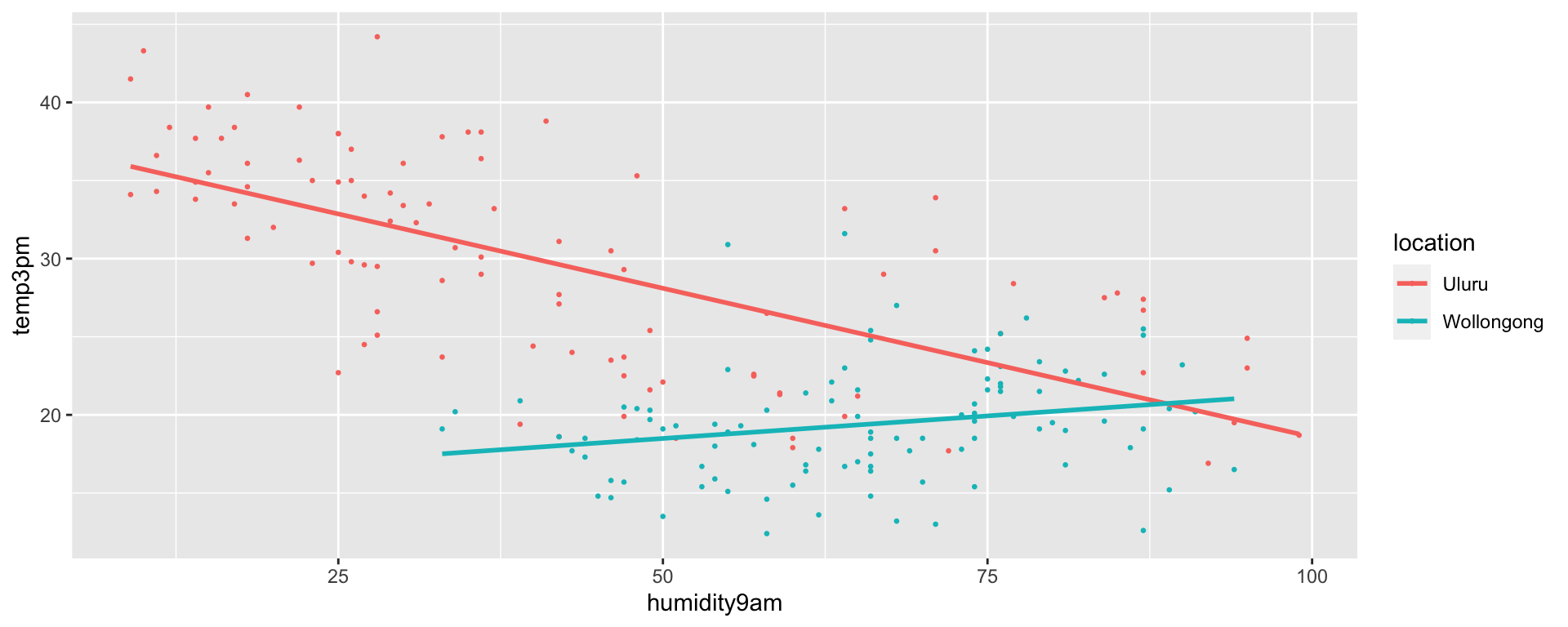
In Uluru, \(X_{i2} = 0\) and the trend in the relationship between 3pm and 9am temperature simplifies to
\[\beta_0 + \beta_1 X_{i1} + \beta_2 \cdot 0 = \beta_0 + \beta_1 X_{i1} \; .\]
In Wollongong, \(X_{i2} = 1\) and the trend in the relationship between 3pm and 9am temperature simplifies to
\[\beta_0 + \beta_1 X_{i1} + \beta_2 \cdot 1 = (\beta_0 + \beta_2) + \beta_1 X_{i1} \; .\]
first_50 <- head(weather_model_3_df, 50)

ggplot(weather_WU, aes(x = temp9am, y = temp3pm)) +
  geom_point(size = 0.01) +
  geom_abline(data = first_50, size = 0.1,
    aes(intercept = `(Intercept)`, slope = temp9am)) +
  geom_abline(data = first_50, size = 0.1,
    aes(intercept = `(Intercept)` + locationWollongong,
    slope = temp9am), color = "blue")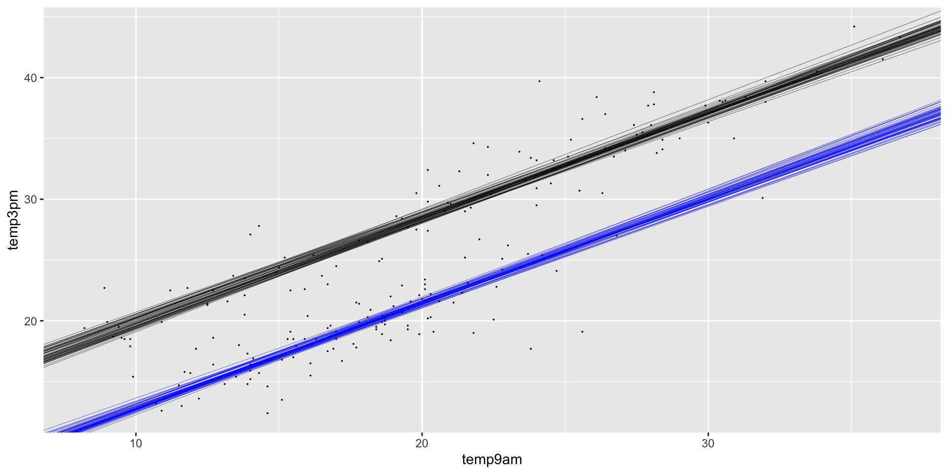
Posterior Predictive Model
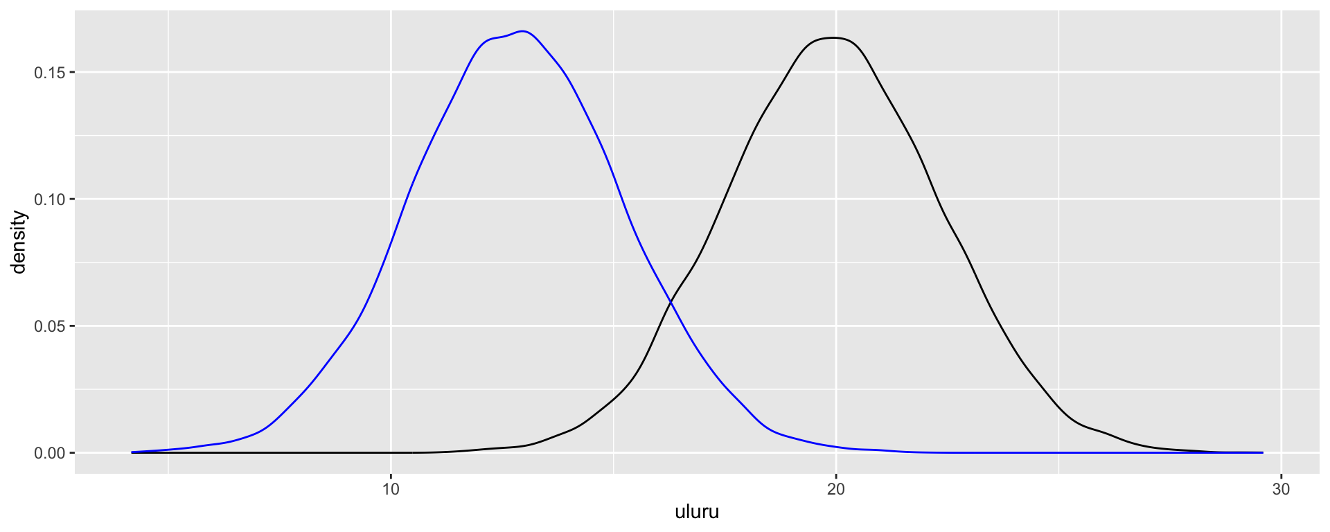
\(\text{likelihood model:}\) \(Y_i | \beta_0, \beta_1, \beta_2, \beta_3 \sigma \;\;\;\stackrel{ind}{\sim} N\left(\mu_i, \sigma^2\right)\text{ with }\) \(\mu_i = \beta_0 + \beta_1X_{i2} + \beta_2X_{i3} + \beta_3X_{i2}X_{i3}\)
\(\text{prior models:}\)
\(\beta_0\sim N(m_0, s_0 )\)
\(\beta_1\sim N(m_1, s_1 )\)
\(\beta_2\sim N(m_2, s_2 )\)
\(\beta_3\sim N(m_3, s_3 )\)
\(\sigma \sim \text{Exp}(l)\)
In Uluru, \(X_{2} = 0\) and the trend in the relationship between temperature and humidity simplifies to
\[\mu = \beta_0 + \beta_2 X_{3} \; .\]
In Wollongong, \(X_{2} = 1\) and the trend in the relationship between temperature and humidity simplifies to
\[\mu = \beta_0 + \beta_1 + \beta_2 X_{3} + \beta_3 X_{3} = (\beta_0 + \beta_1) + (\beta_2 + \beta_3) X_3 \; .\]
model_summary <- summary(interaction_model)
head(as.data.frame(model_summary), -2) %>%
select(`10%`, `50%`, `90%`) %>%
round(3)
10% 50% 90%
(Intercept) 36.419 37.593 38.776
locationWollongong -24.805 -21.883 -18.908
humidity9am -0.215 -0.190 -0.166
locationWollongong:humidity9am 0.198 0.246 0.292
sigma 4.195 4.468 4.772\[\begin{array}{lrl} \text{Uluru:} & \mu & = 37.593 - 0.19 \text{ humidity9am} \\ \text{Wollongong:} & \mu & = (37.593 - 21.883) + (-0.19 + 0.246) \text{ humidity9am}\\ && = 15.71 + 0.056 \text{ humidity9am}\\ \end{array}\]
Do you need an interaction term?
Context.
Visualizations.
Hypothesis tests.
More than two predictors
\(\text{likelihood model:} \; \; \; Y_i | \beta_0, \beta_1,\beta_2,...\beta_p, \sigma \;\;\;\stackrel{ind}{\sim} N\left(\mu_i, \sigma^2\right)\text{ with }\) \(\mu_i = \beta_0 + \beta_1X_{i1} + \beta_2X_{i2} + \ldots +\beta_pX_{ip}\)
\(\text{prior models:}\)
\(\beta_0, \beta_1,\beta_2, ...,\beta_p\sim N(\ldots, \ldots )\)
\(\sigma \sim \text{Exp}(\ldots)\)
Model evaluation and comparison
| Model | Formula |
|---|---|
weather_model_1 |
temp3pm ~ temp9am |
weather_model_2 |
temp3pm ~ location |
weather_model_3 |
temp3pm ~ temp9am + location |
weather_model_4 |
temp3pm ~ . |
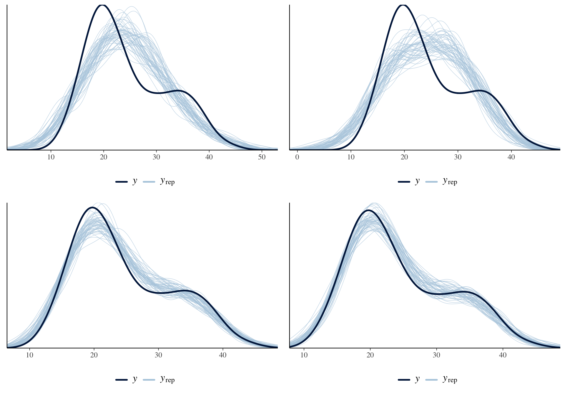
# Posterior predictive models for weather_model_1
ppc_intervals(weather_WU$temp3pm,
  yrep = predictions_1,
  x = weather_WU$temp9am,
  prob = 0.5, prob_outer = 0.95)

# Posterior predictive models for weather_model_2
ppc_violin_grouped(weather_WU$temp3pm,
  yrep = predictions_2,
  group = weather_WU$location,
y_draw = "points")| model | mae | mae scaled | within 50 | within 95 |
| weather model 1 | 3.285 | 0.79 | 0.405 | 0.97 |
| weather model 2 | 3.653 | 0.661 | 0.495 | 0.935 |
| weather model 3 | 1.142 | 0.483 | 0.67 | 0.96 |
| weather model 4 | 1.206 | 0.522 | 0.64 | 0.95 |
