library(tidyverse)
library(lme4) # lme4 package contains sleep study data
data(sleepstudy)
baseline <- sleepstudy %>%
  filter(Days==2) # Day 2 is baseline, days 0-1 are training
baseline %>%
  ggplot(aes(x=Reaction)) +
  geom_histogram() +
  labs(x="Reaction Time (ms)") +
geom_vline(xintercept=275, col="red")Posterior Analysis
with MCMC and rstanarm
Day 3
Reaction Times
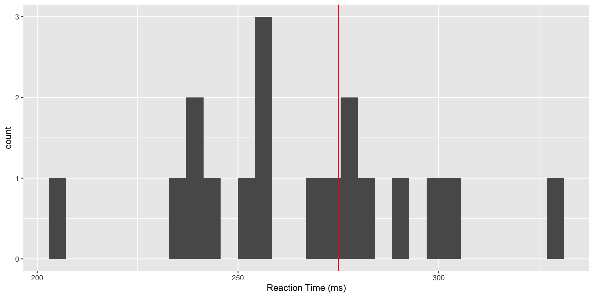
We consider data from a study (Belenky et al, 2003) of reaction time under a variety of sleep deprivation scenarios. We will focus on the baseline values of reaction time, taken after study participants had a normal night’s sleep. Suppose prior research has established a mean reaction time to a visual stimulus of 275ms, and we wish to determine whether the values in our study are consistent with this value. A first step is to read and plot the data.
Reaction Time Data
Analysis of Reaction Time
We can use the R brms() function to analyze the data. One advantage of this function is that it allows us easily to implement more complex sampling algorithms, beyond Gibbs sampling.
Suppose our data model is \(Y \sim N(\mu, \sigma^2),\) and we wish to evaluate whether \(\mu\) is consistent with a reaction time of 275ms. We previously studied the conjugate normal-inverse gamma specification, given by \[\mu \mid \sigma^2 \sim N\bigg(\theta,\frac{\sigma^2}{n_0}\bigg), ~~~\frac{1}{\sigma^2} \sim \text{gamma}\bigg(\frac{\nu_0}{2},\frac{\nu_0\sigma^2_0}{2}\bigg).\] While this prior has a nice interpretation in terms of prior samples, it’s not the only option.
Prior for the Mean
Instead, we consider a relatively non-informative prior for our mean \(\mu \sim N(300,50^2)\) – based on a normal distribution, this puts 95% of the prior mass within 2 SD of the mean, which roughly corresponds to the range 200-400.
Prior for the Standard Deviation
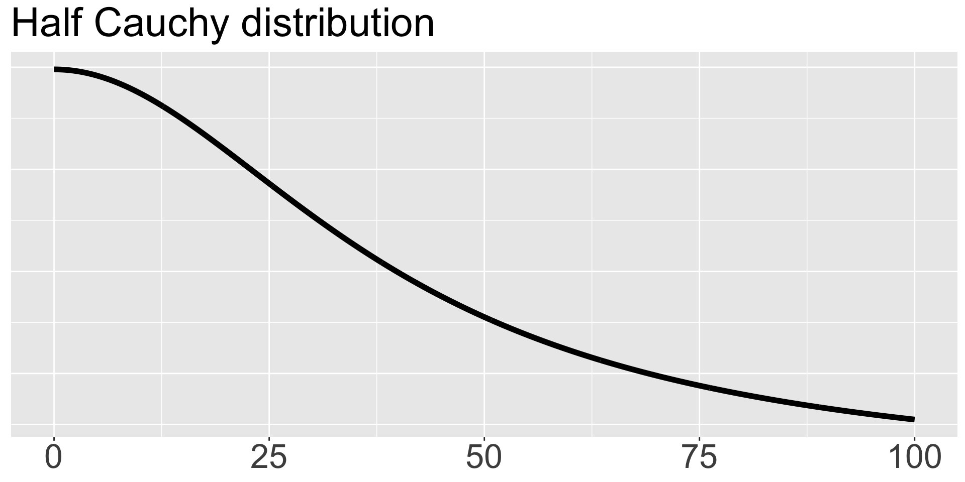
We will specify a prior directly on the standard deviation \(\sigma\) as \(\sigma \sim \text{HalfCauchy}(0,40)\), which has mean 0 and scale parameter 40 and is called “half” because only the positive values are used. If you haven’t seen the Cauchy distribution, it’s a special case of a t distribution with 1 degree of freedom, and it’s nice because it has fat tails and allows substantial mass away from its mean. We plot it here.
Code to Fit Model
fit <- stan_glm(data = baseline, family = gaussian,
                Reaction ~ 1, #only estimating a mean (Intercept) and variance
                prior_intercept = normal(300, 50),
                # prior for mu has mean 300 and sd 50
                prior_aux = cauchy(0, 40),
                # prior for sigma is half of a center 0, scale 40 Cauchy
                chains = 4, iter = 5000*2, seed = 84735, refresh = FALSE
)
Checking the Output
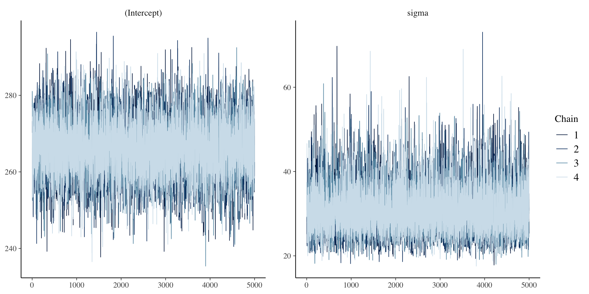
Trace plots can be used to check convergence.
Checking the Output
Interpreting Trace Plots
A trace plot depicts the MCMC samples by MCMC iteration number. If your MCMC algorithm has converged, we expect to see trace plots that reflect white noise around the target value. Indeed, that appears to be the case here.
Bad Trace Plots
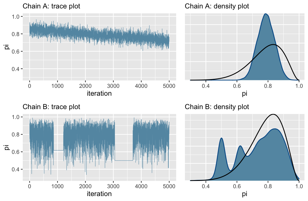
Chain A has not yet converged to the right value (see black line in density plot), while Chain B is getting stuck and moving slowly around the sample space. In these cases, think carefully about your model and make sure it’s appropriate, and if so, try sampling a larger number of iterations.
Comparing Sampled Values Across Chains
We also can check the \(\hat{R}\) values. These compare the sampled values across chains (we hope all the chains are giving similar results) by taking the square root of the ratio of the variability in the parameter of interest across all chains combined to the typical variability within a given chain. When \(\hat{R} \approx 1\), we have stability across the chains. While there is no universal rule, often \(\hat{R}>1.05\) can be a cause for concern.
Checking \(\hat{R}\)
Effective Sample Size
Markov chain simulations in general produce samples that are correlated, rather than independent. The degree of autocorrelation in samples is related to the speed of convergence of the chain. The effective sample size (ESS) is the number of independent samples you would need to get a similarly accurate posterior approximation. An effective sample size much smaller than the actual number of samples in a chain is an indication that our sampling is not very efficient. Depending on software courses, we may see one ESS for each parameter, or two values describing ESS in the center and tails of the distribution for each parameter.
Effective Sample Size
The bulk ESS provides information about the sampling efficiency in the bulk of the distribution and is thus most relevant for providing information about efficiency of mean or median estimates. (brms)
Tail ESS computes the minimum of ESS of the 5% and 95% quantiles and is useful for determining sampling efficiency in the tails and of the variance. (brms)
ESS can also be calculated overall for each parameter (rstanarm)
There are no hard and fast rules, but one recommendation is that both values should be at least 100 per Markov chain.
Generally, we evalute quality of our samples based on all these criteria combined.
Effective Sample Size
(Intercept)       sigma
     0.5448      0.5251
Evaluating Our Hypothesis
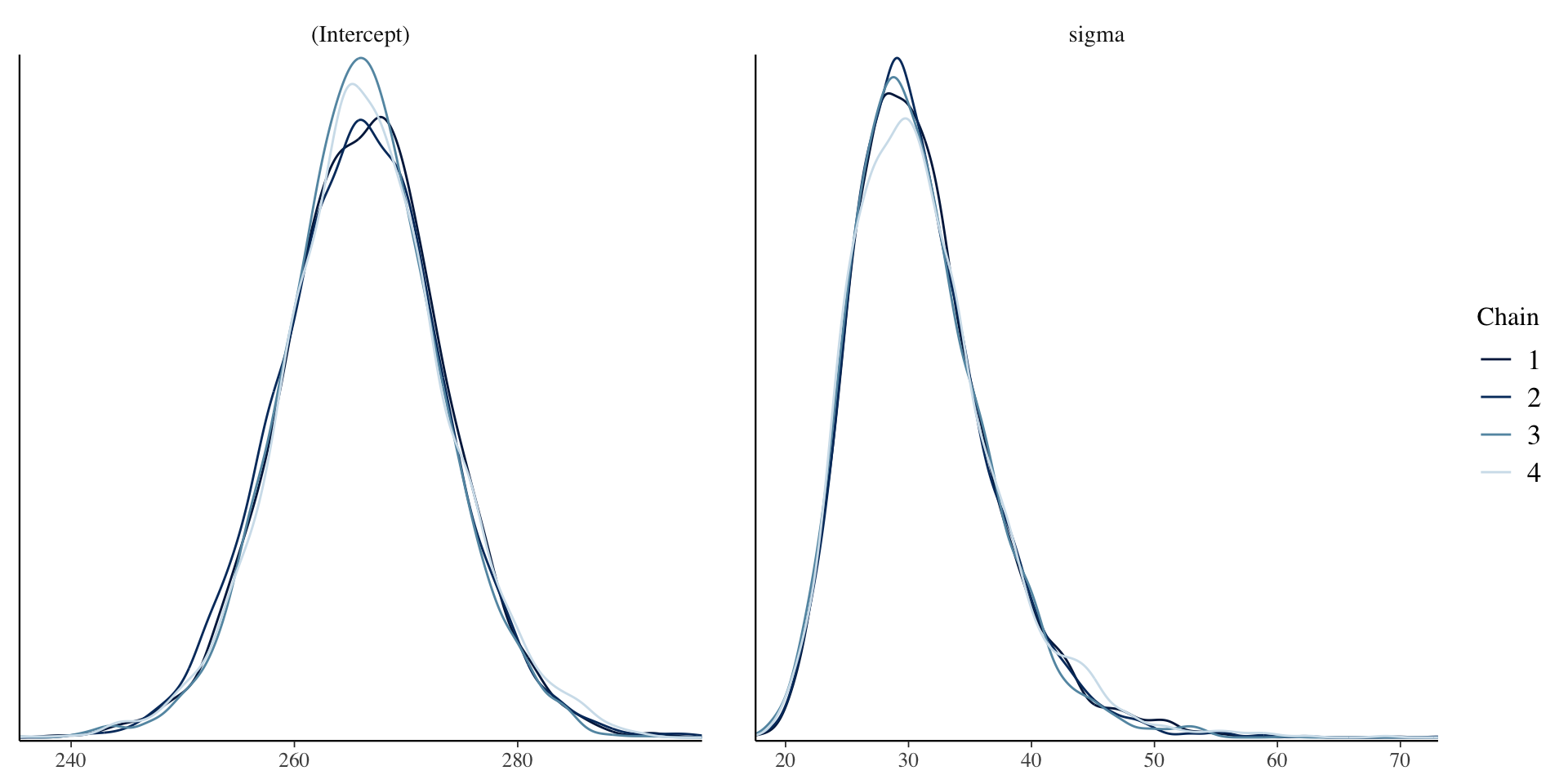
Examining the posterior distribution for \(\mu\), we see that most of its mass is below the value 275.
We can easily calculate the posterior probability that \(\mu<275\) by taking the fraction of posterior samples that are less than 275.
So the posterior probability that \(\mu<275\) is 0.8917.
Evaluating Our Hypothesis
tidy(fit,
     effects = c("fixed", "aux"),
     conf.int = TRUE,
     conf.level = 0.95) # written summary of the output
# A tibble: 3 × 5
term estimate std.error conf.low conf.high
<chr> <dbl> <dbl> <dbl> <dbl>
1 (Intercept) 266. 6.97 252. 281.
2 sigma 30.3 5.65 22.3 44.2
3 mean_PPD 266. 10.4 246. 287. We can also use the 95% credible interval for \(\mu\) and note that 275 is inside this credible interval.
You Try It!
The priors specified are not very informative. Try making the priors more informative and running the code on your own to see how the results are affected!
For example, you can - make the variance on the normal prior much smaller - make the scale on the half Cauchy prior much smaller
Try changing just one aspect of the prior at a time to evaluate robustness.
Changes in Reaction Time with Sleep Deprivation
Now that we’ve explored baseline reaction time, let’s see what happens to the reaction times of study participants after one night of sleep deprivation (only 3 hours of time in bed). First, we will do a little data wrangling and make a plot of the changse in reaction time, plotting the sleep deprived reaction time minus the baseline reaction time for each subject.
Changes in Reaction Time
sleepdep <- sleepstudy %>%
  filter(Days %in% c(2,3)) %>%
  pivot_wider(names_from = Days, names_prefix="Day",
              values_from = Reaction, id_cols=Subject) %>%
  mutate(diff32=Day3-Day2)
  # consider day 2 baseline and day 3, the first value from a sleep-deprived state, and calculate difference
  # positive differences indicate longer reaction times when sleep-deprived
sleepdep %>%
  ggplot(aes(x=diff32)) +
  geom_histogram() +
  labs(x="Difference in Reaction Time (ms) when Sleep Deprived") +
  geom_vline(xintercept=0, col="red")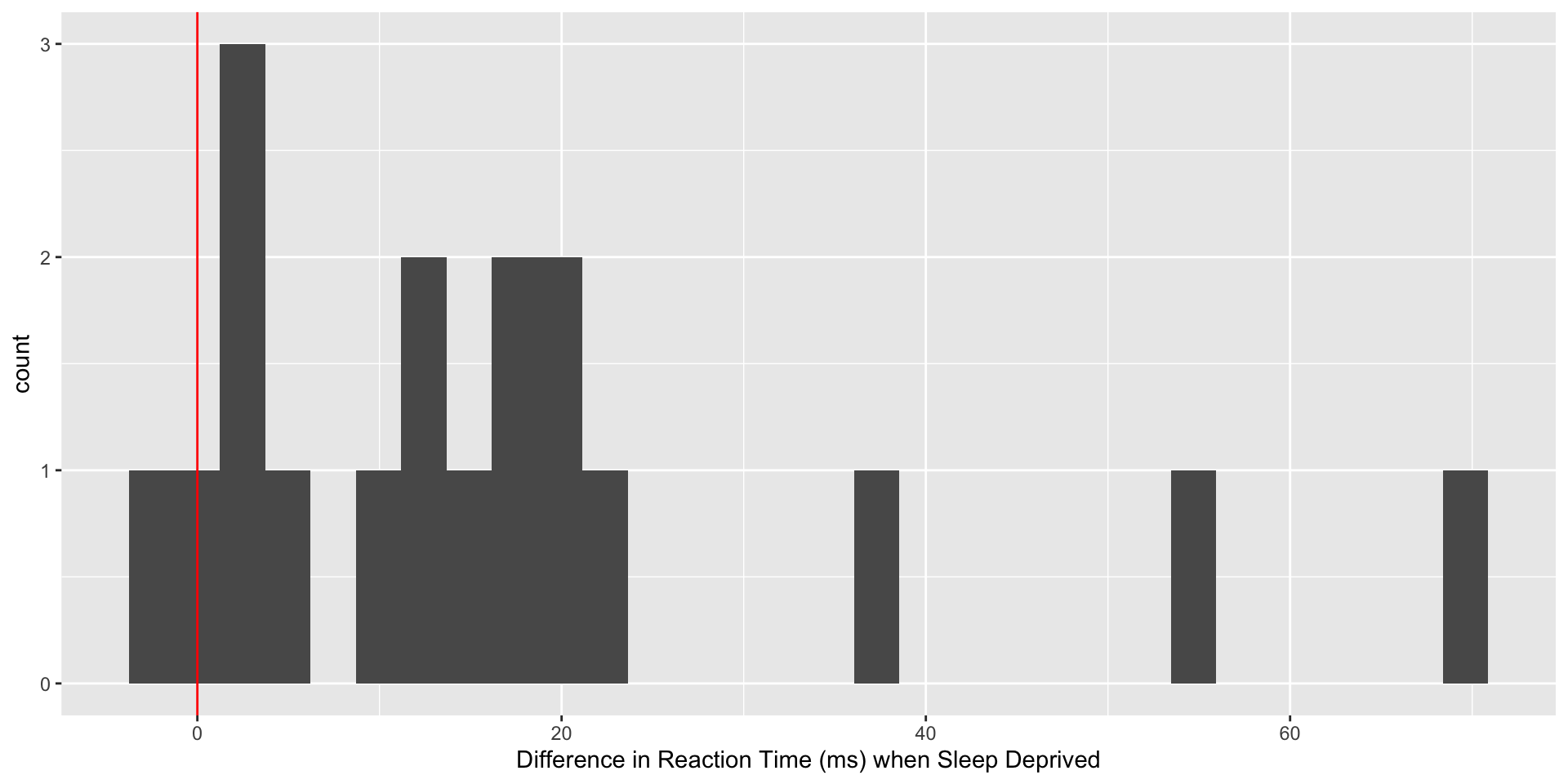
You Try It!
Using the previous slides as a guide, evaluate the hypothesis that sleep deprivation increases reaction time.
Warning
Think carefully about your priors!
