Conjugate Priors and their Posteriors
Day 2
Note that this lecture is based in part on Chapter 5 of Bayes Rules! book.
Review Application
California Drought
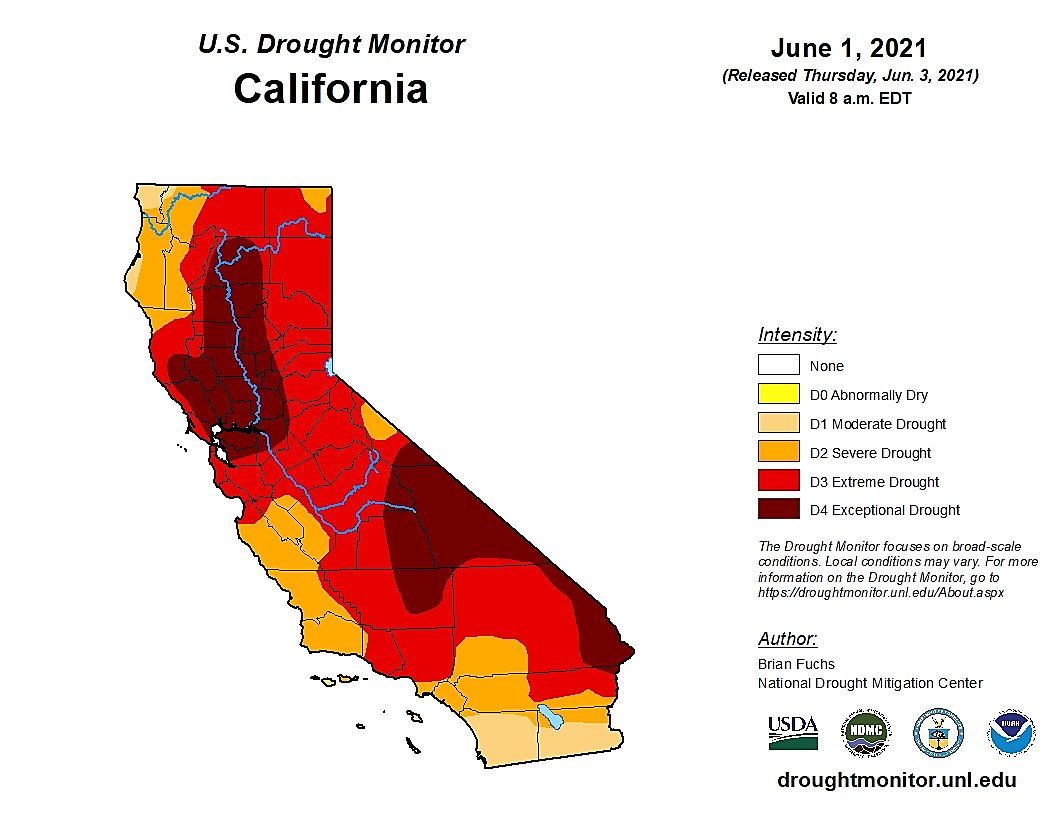
Drought conditions have been a major concern for California residents and policy makers for years. We consider historical data on “extremely dry years” to formulate a prior distribution – for example, from 1900-1999, 42 years were characterized as “extremely dry.” For data analysis, we will assume we go back in time to 2020 and let data from 2020, 2021, and 2022 contribute to our data likelihood.
Prior Distribution Options
We can use a beta prior based on the historical data from 1900-1999, during which we had 42 years that were extremely dry, and 58 years that were not. This corresponds to a beta(42,58) prior distribution (remember, the parameters of the beta can be interpreted as prior data: the approximate # of prior dry and non-dry years). Let’s plot and summarize this prior.
  mean      mode         var         sd
1 0.42 0.4183673 0.002411881 0.04911091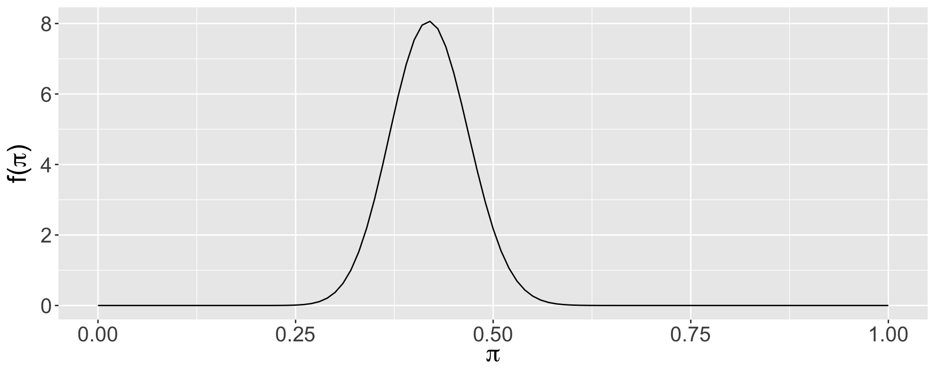
Does this seem reasonable?
Priors for Drought
California weather has been more variable in recent years, and you may not all agree on an appropriate prior distribution.
| Time | Historical Data | Prior Model |
|---|---|---|
| 1900-1999 | 42 extremely dry years | Beta(42,58) |
| 2000-2009 | 9 extremely dry years | Beta(9,1) |
| 2010-2019 | 7 extremely dry years | Beta(7,3) |
| NA | Vague prior not based on data | Beta(1,1) |
Pick one of these prior models, or design your own, and plot your prior. Share your plot with colleagues!
2020
| Prior Model | Data | Posterior Model |
|---|---|---|
| Beta(?,?) | Extremely dry year | Beta(?,?) |
| Prior Type | Prior Model | Data | Posterior Model |
|---|---|---|---|
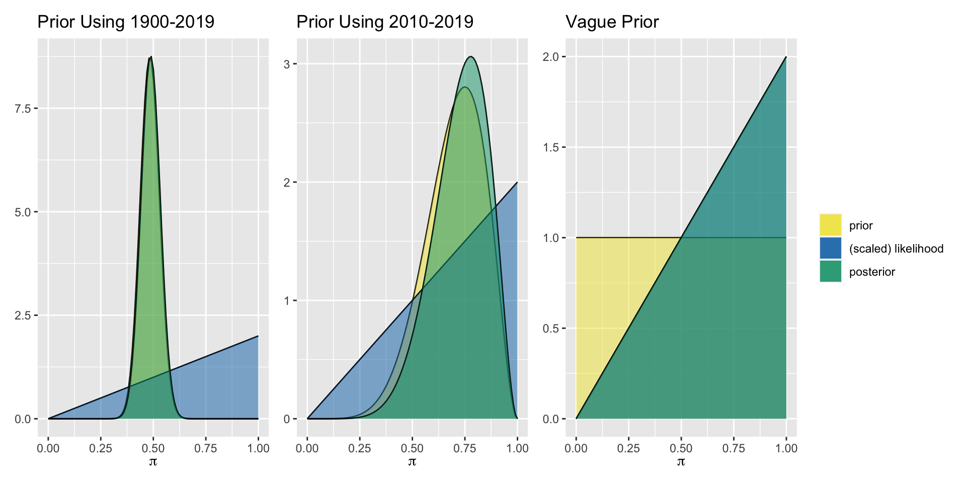
| 1900-2019 | Beta(58, 62) | Extremely dry year | Beta(59,62) |
| Last 10 years | Beta(7,3) | Extremely dry year | Beta(8,3) |
| Agnostic | Beta(1,1) | Extremely dry year | Beta(2,1) |
Aside: More Informative Prior
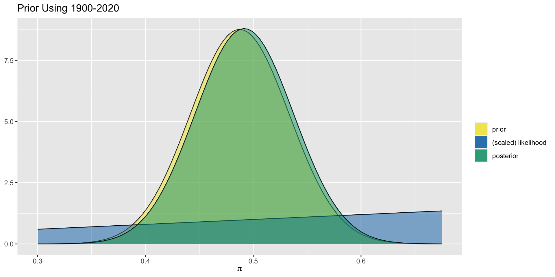
For the more informative prior, using 121 years of historical data, the prior and posterior are not exactly the same but are very close. We can focus in more closely to see the slight difference.
Aside: Posterior Proportional to Likelihood
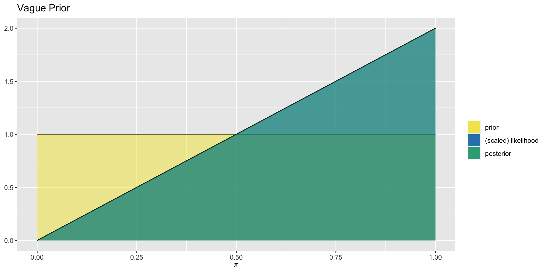
For the uniform prior distribution, the prior takes the same value everywhere, so the posterior distribution (generally proportional to the prior times the likelihood) is simply proportional to the likelihood.
2021
Now, take your posterior and use it as the prior distribution for analysis of the data from 2021.
2021
| Prior Model | Data | Posterior Model |
|---|---|---|
| Beta(?,?) | Extremely dry year | Beta(?,?) |
| Prior Type | Prior Model | Data | Posterior Model |
|---|---|---|---|
| 1900-2020 | Beta(59, 62) | Extremely dry year | Beta(60,62) |
| Last 11 years | Beta(8,3) | Extremely dry year | Beta(9,3) |
| Agnostic | Beta(2,1) | Extremely dry year | Beta(3,1) |
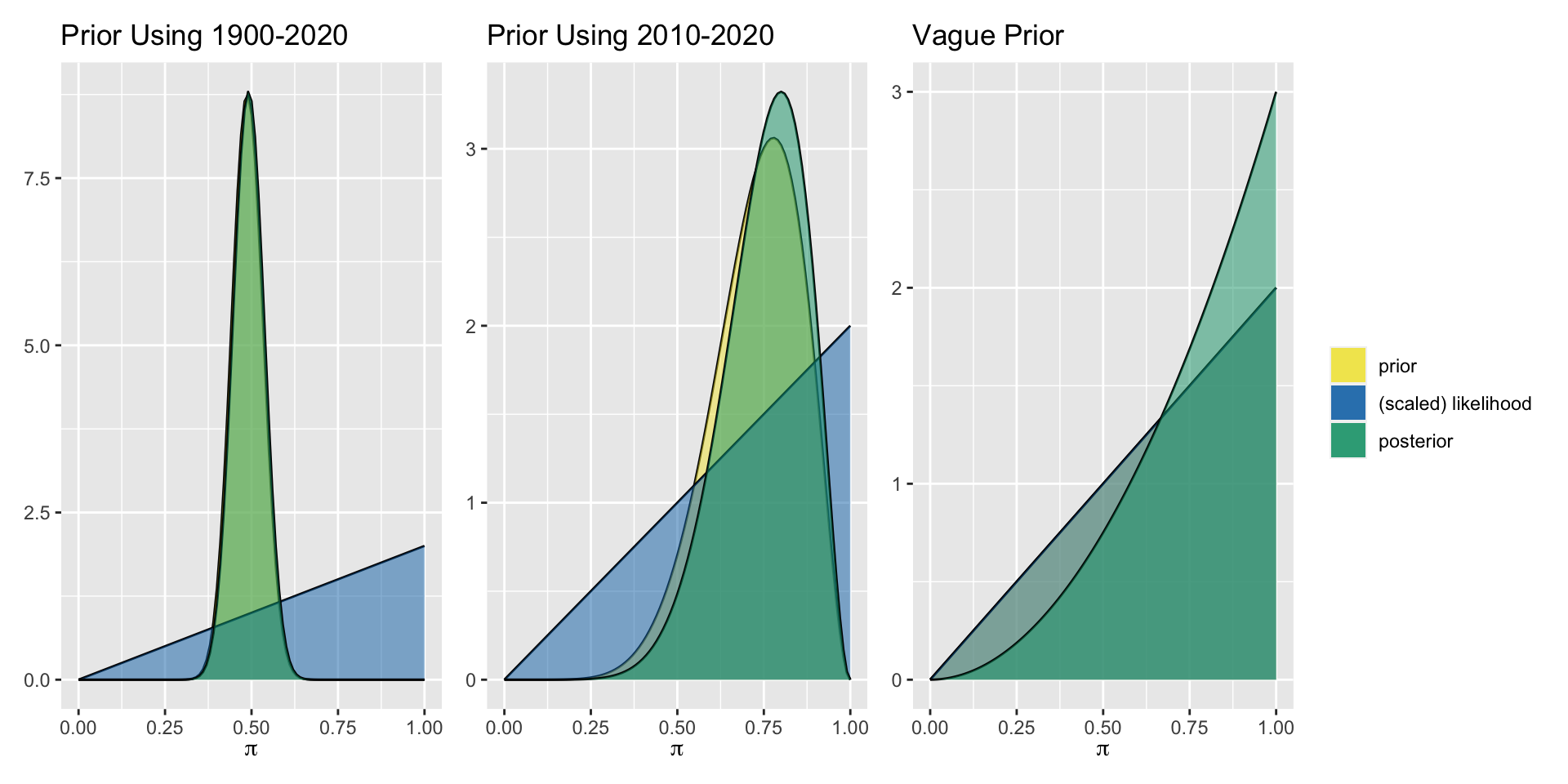
Aside: Posterior Proportional to Likelihood
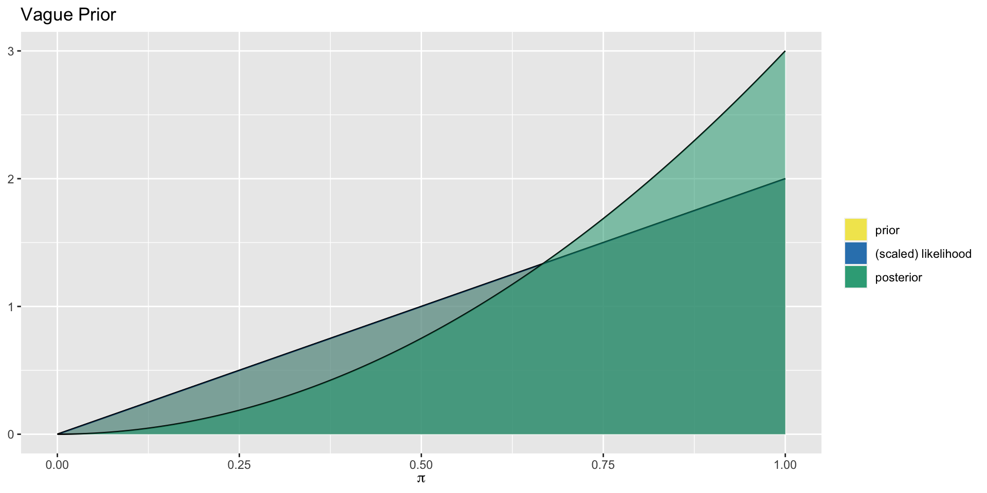
In this case, the prior Beta(2,1) is proportional to \(\pi^{2-1}(1-\pi)^{1-1}=\pi\), and the likelihood is also proportional to \(\pi^1(1-\pi)^0=\pi\).
2022
Finally, take your posterior and use it as the prior distribution for analysis of the data from 2022.
2022
| Prior Model | Data | Posterior Model |
|---|---|---|
| Beta(?,?) | Extremely dry year | Beta(?,?) |
| Prior Type | Prior Model | Data | Posterior Model |
|---|---|---|---|
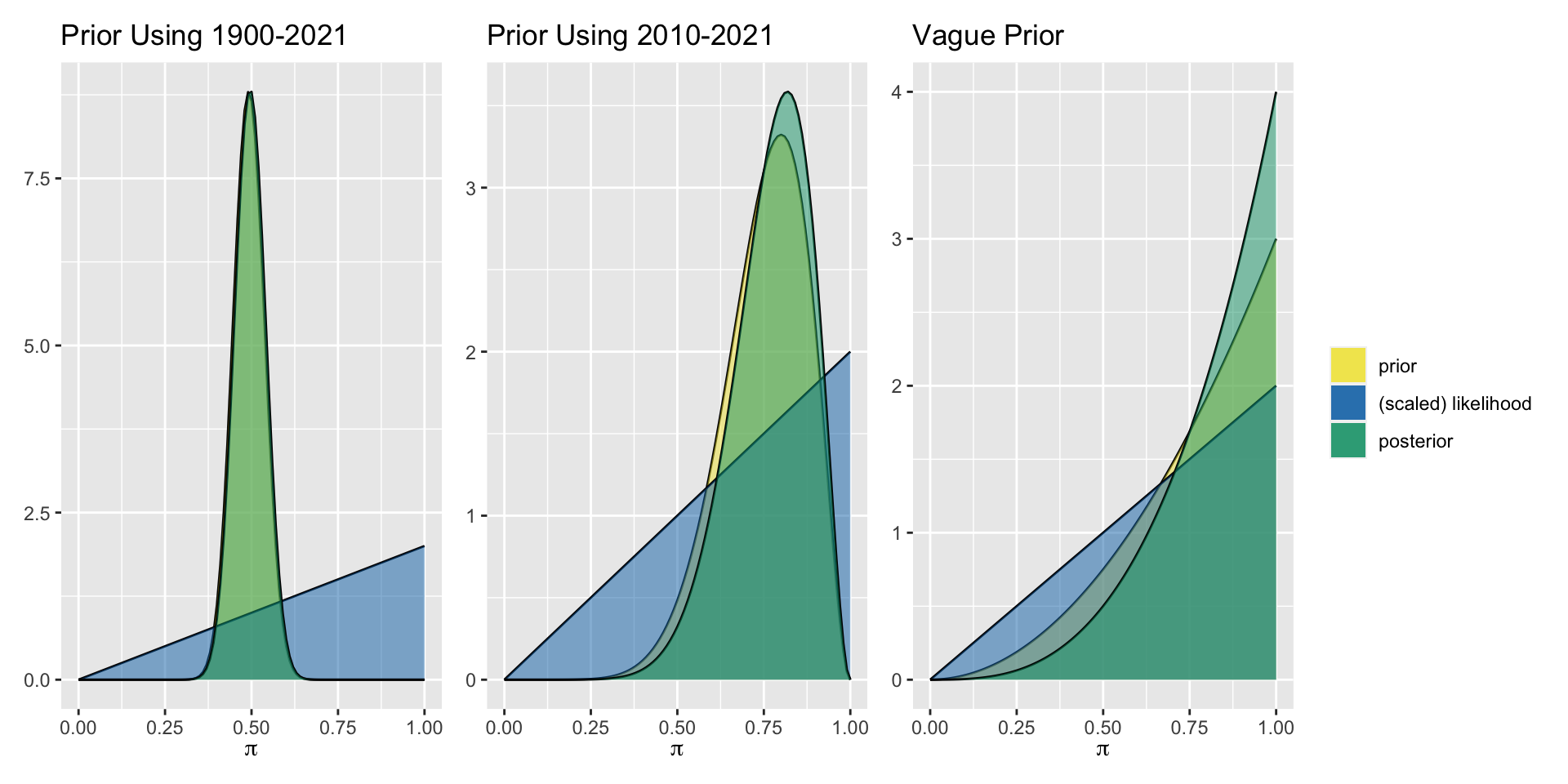
| 1900-2021 | Beta(60, 62) | Extremely dry year | Beta(61,62) |
| Last 12 years | Beta(9,3) | Extremely dry year | Beta(10,3) |
| Agnostic | Beta(3,1) | Extremely dry year | Beta(4,1) |
Continuous Response Data: The Normal-Normal Model
Data
Example from bayesrulesbook.com
Let \((Y_1,Y_2,\ldots,Y_{25})\) denote the hippocampal volumes for the \(n = 25\) study subjects who played collegiate American football and who have been diagnosed with concussions:
Data
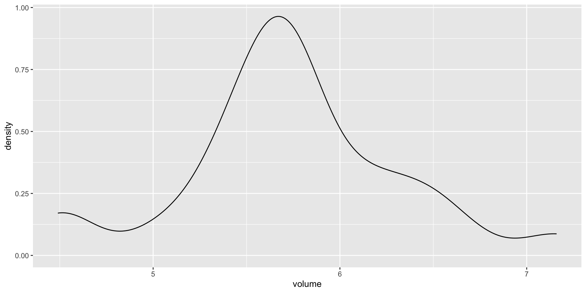
The Normal Model
Let \(Y\) be a random variable which can take any value between \(-\infty\) and \(\infty\), ie. \(Y \in (-\infty,\infty)\). Then the variability in \(Y\) might be well represented by a Normal model with mean parameter \(\mu \in (-\infty, \infty)\) and standard deviation parameter \(\sigma > 0\):
\[Y \sim N(\mu, \sigma^2)\]
The Normal model is specified by continuous pdf
\[\begin{equation} f(y) = \frac{1}{\sqrt{2\pi\sigma^2}} \exp\bigg[{-\frac{(y-\mu)^2}{2\sigma^2}}\bigg] \;\; \text{ for } y \in (-\infty,\infty) \end{equation}\]
Trends and Variability of the Normal Model
\[\begin{split} E(Y) & = \text{ Mode}(Y) = \mu \\ \text{Var}(Y) & = \sigma^2 \\ \end{split}\]
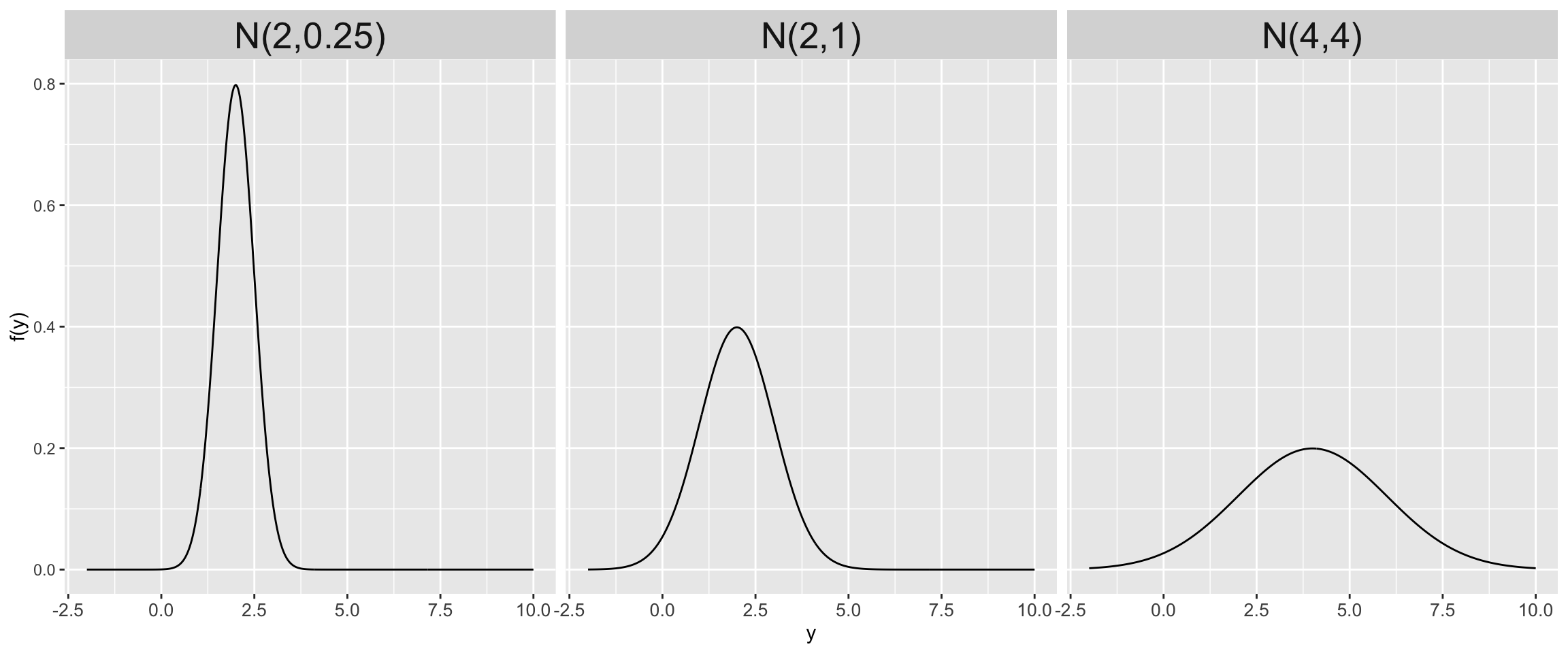
Further, \(\sigma\) provides a sense of scale for \(Y\). Roughly 95% of \(Y\) values will be within 2 standard deviations of \(\mu\):
\[\begin{equation} \mu \pm 2\sigma \; . \end{equation}\]
Normal models
Normal Likelihood
\[L(\mu |\vec{y})= \prod_{i=1}^{n}L(\mu | y_i) = \prod_{i=1}^{n}\frac{1}{\sqrt{2\pi\sigma^2}} \exp\bigg[{-\frac{(y_i-\mu)^2}{2\sigma^2}}\bigg].\]
Simplifying this up to a proportionality constant
\[L(\mu |\vec{y}) \propto \prod_{i=1}^{n} \exp\bigg[{-\frac{(y_i-\mu)^2}{2\sigma^2}}\bigg] = \exp\bigg[{-\frac{\sum_{i=1}^n (y_i-\mu)^2}{2\sigma^2}}\bigg] \; .\]
\[\begin{equation} L(\mu | \vec{y}) \propto \exp\bigg[{-\frac{(\bar{y}-\mu)^2}{2\sigma^2/n}}\bigg] \;\;\;\; \text{ for } \; \mu \in (-\infty, \infty). \end{equation}\]
\[L(\mu | \vec{y}) \propto \exp\bigg[{-\frac{(5.735-\mu)^2}{2(0.593^2/25)}}\bigg] \;\;\;\; \text{ for } \; \mu \in (-\infty, \infty),\]
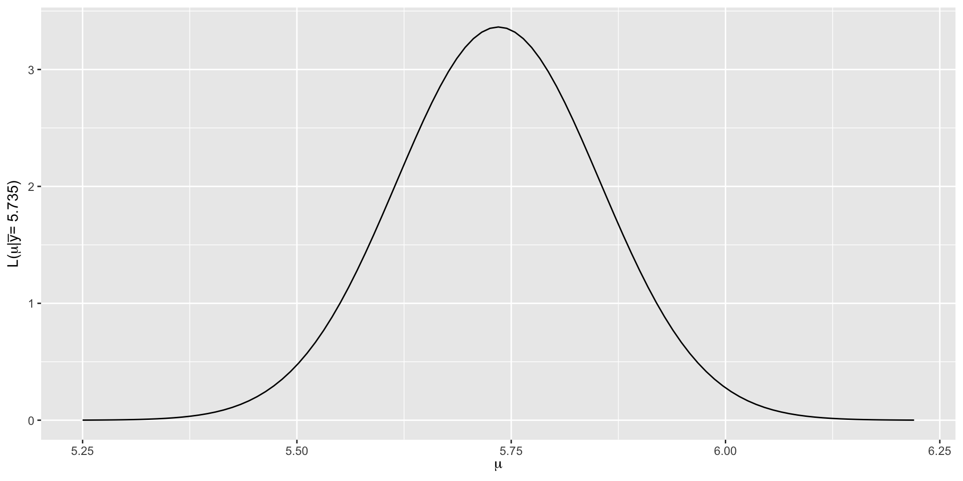
The joint Normal likelihood function for the mean hippocampal volume.
Normal Prior for the Mean
\[\mu \sim N(\theta, \tau^2) \; , \]
with prior pdf
\[\begin{equation} f(\mu) = \frac{1}{\sqrt{2\pi\tau^2}} \exp\bigg[{-\frac{(\mu - \theta)^2}{2\tau^2}}\bigg] \;\; \text{ for } \mu \in (-\infty,\infty) \; . \end{equation}\]
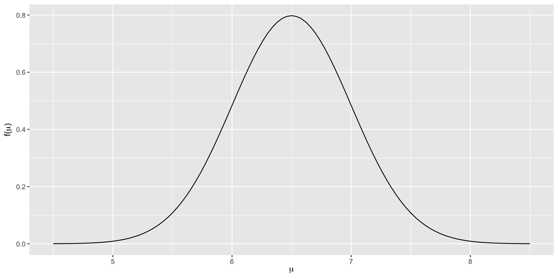
Wikipedia tells us that among the general population of human adults, both halves of the hippocampus have a volume between 3.0 and 3.5 cubic centimeters. Thus the total hippocampal volume of both sides of the brain is between 6 and 7 cubic centimeters. A standard deviation \(\sigma=0.5\) for a normal prior centered at 6.5 puts about 2/3 of the mass of the prior in this range: \(\mu \sim N(6.5, 0.5^2) \;.\)
\(N(6.5, 0.5^2)\) Distribution
The Normal-Normal Bayesian Model
Let \(\mu \in (-\infty,\infty)\) be an unknown mean parameter and \((Y_1,Y_2,\ldots,Y_n)\) be an independent \(N(\mu,\sigma^2)\) sample where \(\sigma\) is assumed to be known (we’ll relax this strong assumption shortly). The Normal-Normal Bayesian model complements the Normal structure of the data with a Normal prior on \(\mu\):
\[\begin{split} Y_i | \mu & \stackrel{ind}{\sim} N(\mu, \sigma^2) \\ \mu & \sim N(\theta, \tau^2) \\ \end{split}\]
Upon observing data \(\vec{y} = (y_1,y_2,\ldots,y_n)\), the posterior model of \(\mu\) is \(N(\mu_n,\tau^2_n)\).
Normal Posterior
In the posterior \(N(\mu_n,\tau^2_n)\), we have \[\mu_n=\frac{\bigg(\frac{1}{\tau^2}\bigg)\theta+\bigg(\frac{n}{\sigma^2}\bigg)\bar{y}}{\frac{1}{\tau^2}+\frac{n}{\sigma^2}}\] and \[\tau^2_n=\frac{1}{\frac{1}{\tau^2}+\frac{n}{\sigma^2}}.\]
The inverse variance \(\frac{1}{\tau^2_n}\) is also called the precision. Note \(\frac{1}{\tau^2_n}=\frac{1}{\tau^2}+\frac{n}{\sigma^2}\) and thus the posterior precision is the prior precision (inverse variance) combined with the inverse data variance (information).
Posterior Mean as Weighted Average of Prior and Sample Means
Now \[\mu_n=\frac{\bigg(\frac{1}{\tau^2}\bigg)\theta+\bigg(\frac{n}{\sigma^2}\bigg)\bar{y}}{\frac{1}{\tau^2}+\frac{n}{\sigma^2}}.\]
Notice that the posterior mean is a weighted average of the prior mean and the sample mean, with the prior mean weighted by the prior precision, and the sample mean weighted by its sampling precision.
Back to Brains
For the hippocampus data, we selected the prior \(\mu \sim N(6.5, 0.5^2)\), and recall in our dataset the mean was 5.735 and sd was 0.593.
The posterior model of \(\mu\) is:
\[\mu | \vec{y} \; \sim \; N\bigg(\frac{6.5*\frac{1}{0.5^2} + 5.735*\frac{25}{0.593^2}}{\frac{1}{0.5^2}+\frac{25}{0.593^2}}, \; \frac{1}{\frac{1}{0.5^2}+\frac{25}{0.593^2}}\bigg)\;,\]
or, further simplified,
\[\mu | \vec{y} \; \sim \; N\bigg(5.776, 0.115^2 \bigg) \; .\]
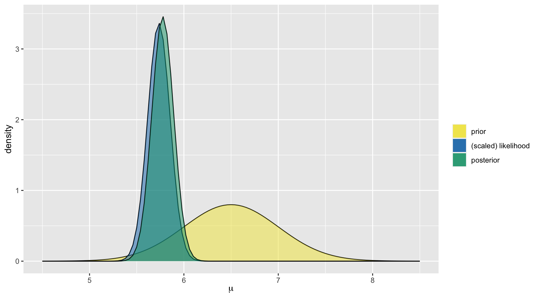
      model     mean     mode        var        sd
1     prior 6.500000 6.500000 0.25000000 0.5000000
2 posterior 5.775749 5.775749 0.01331671 0.1153981
Interpretation of Conjugate Prior in Terms of Historical Data
If we base our prior mean on \(n_0\) observations from a similar population as \((Y_1,Y_2,\ldots,Y_n)\), we may wish to set \(\tau^2=\frac{\sigma^2}{n_0}\), the variance of the mean of the prior observations. In this case, we can simplify our equation as
\[\mu_n=\frac{\bigg(\frac{1}{\tau^2}\bigg)\theta+\bigg(\frac{n}{\sigma^2}\bigg)\bar{y}}{\frac{1}{\tau^2}+\frac{n}{\sigma^2}} = \frac{\bigg(\frac{n_0}{\sigma^2}\bigg)\theta+\bigg(\frac{n}{\sigma^2}\bigg)\bar{y}}{\frac{n_0}{\sigma^2}+\frac{n}{\sigma^2}}\] \[\mu_n= \bigg(\frac{n_0}{n_0+n}\bigg)\theta + \bigg(\frac{n}{n_0+n}\bigg)\bar{y},\] so we see our conjugate prior has an interpretation in terms of historical data when \(\theta\) is the prior mean in a sample of size \(n_0\).
Known \(\sigma^2\)?
When is \(\sigma^2\) actually known? Well, pretty much never. This case is primarily used for didactic purposes.
Conjugate Inference in Normal-Normal Model with \(\sigma^2\) Unknown
Typically, we make joint inference for the mean and variance. Using probability axioms, we express a joint distribution as a product of a conditional probability and a marginal probability, e.g. \[f(\mu,\sigma^2)=f(\mu \mid \sigma^2)f(\sigma^2).\]
Prior for \(\sigma^2\)
For \(\sigma^2\), we need a prior with support on \((0,\infty)\). One nice option is the gamma distribution. While this distribution is not conjugate for \(\sigma^2\), it is conjugate for the precision, \(\frac{1}{\sigma^2}\)
The gamma distribution is parameterized in terms of a shape parameter \(\alpha\) and rate parameter \(\beta\) and has mean \(\frac{\alpha}{\beta}\) and variance \(\frac{\alpha}{\beta^2}\).
We write these prior models as \(\frac{1}{\sigma^2} \sim \text{gamma}(\alpha,\beta)\) or equivalently \(\sigma^2 \sim \text{inverse-gamma}(\alpha,\beta)\).
Gamma Models
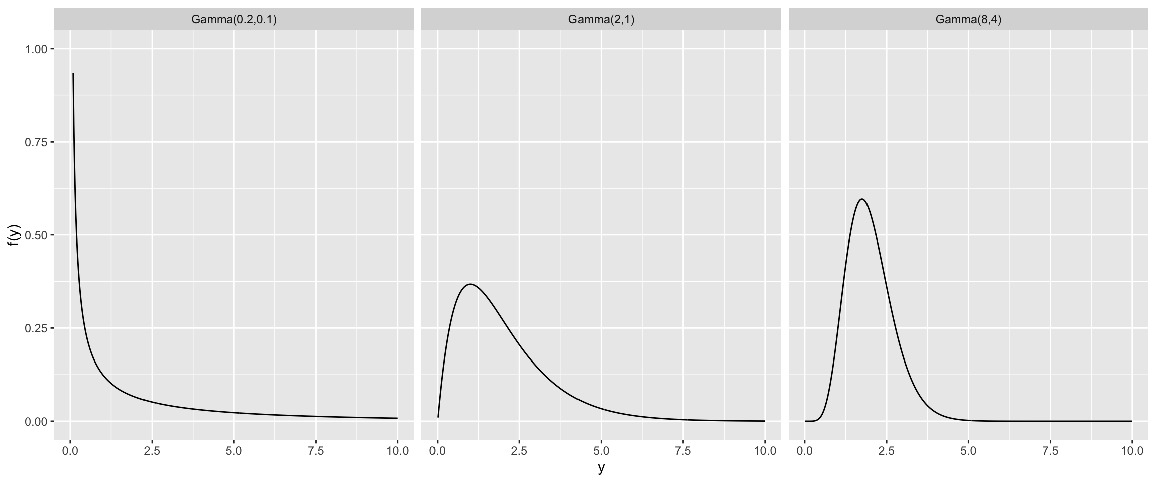
Suppose we think the variance should be centered around \(\frac{1}{2}\). Here are some gamma priors (for the precision) all with mean \(2=\frac{1}{0.5}\).
Interpretable Gamma Prior Model for Precision
Recall the \(\text{gamma}(\alpha,\beta)\) prior has mean \(\frac{\alpha}{\beta}\). One way to pick \(\alpha\) and \(\beta\) would be to center the prior on an existing estimate of the precision. So for interpretability, we can set \[\frac{1}{\sigma^2} \sim \text{gamma}\bigg(\frac{\nu_0}{2},\frac{\nu_0\sigma^2_0}{2}\bigg),\] where we interpret \(\sigma^2_0\) as the sample variance from a sample of prior observations of size \(\nu_0\).
This prior for the precision has mean \(\frac{1}{\sigma^2_0}\).
Normal-Inverse Gamma Conjugate Prior Model
When our priors are \[\frac{1}{\sigma^2} \sim \text{gamma}\bigg(\frac{\nu_0}{2},\frac{\nu_0\sigma^2_0}{2}\bigg)\] and \[\mu \mid \sigma^2 \sim N\bigg(\theta,\frac{\sigma^2}{n_0}\bigg), \] and our data model is \[Y_1, \ldots, Y_n \mid \mu, \sigma^2 \sim N(\mu,\sigma^2)... \]
Normal-Inverse Gamma Conjugate Prior Model
… we have a conjugate prior for the variance and a conditionally-conjugate prior for the mean. The full conditional posterior for \(\mu\) is \[\mu \mid Y_1, \ldots, Y_n, \sigma^2 \sim N\bigg(\mu_n, \frac{\sigma^2}{n*}\bigg),\] where \(n^*=n_0+n\) and \(\mu_n=\frac{\frac{n_0}{\sigma^2}\theta+\frac{n}{\sigma^2}\bar{y}}{\frac{n_0}{\sigma^2}+\frac{n}{\sigma^2}}=\frac{n_0\theta+n\bar{y}}{n^*}.\)
With \(\theta\) viewed as the mean of \(n_0\) prior observations, then \(E(\mu \mid Y_1, \ldots, Y_n,\sigma^2)\) is the sample mean of the current and prior observations, and \(\text{Var}(\mu \mid Y_1, \ldots, Y_n, \sigma^2)\) is \(\sigma^2\) divided by the total number of observations (prior+current).
Normal-Inverse Gamma Conjugate Prior Model
To get the marginal posterior of \(\sigma^2\), we integrate over the unknown value of \(\mu\) and obtain \[\frac{1}{\sigma^2} \mid Y_1, \ldots, Y_n \sim \text{gamma}\bigg(\frac{\nu_n}{2},\frac{\nu_n \sigma^2_n}{2}\bigg),\] where \(\nu_n=\nu_0+n\), \[\sigma^2_n=\frac{1}{\nu_n}\bigg[\nu_0\sigma^2_0 + (n-1)s^2 + \frac{n_0n}{n^*}(\bar{y}-\theta)^2\bigg],\] where \(s^2=\frac{\sum_{i=1}^n (y_i-\bar{y})^2}{n-1}\) is the sample variance.
